Fluorescence - [work in progress]

Fluorescence serves as a proxy for numerous essential ocean variables (EOV). Its measurement is to study both biological and physical oceanographic phenomena.

The “Background” section summarizes the general principles of fluorescence, its applications in oceanography, and relevant measurement units and standards. The Sensing section covers core optical methods and associated techniques. Some fluorescence sensors and DIY project are listed in the available sensors section.

Contributions:

• Olivier Fauvarque, Morgane Tardivel, [Clothilde Haristoy], Dewi Langlet, Adèle Moncuquet

---

Background

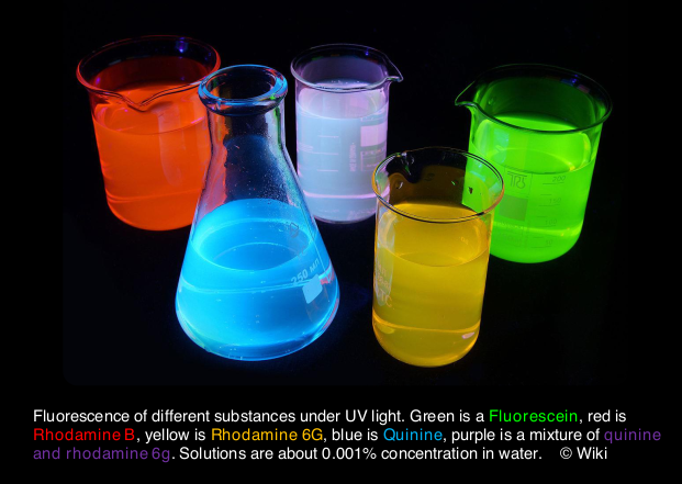
Figure 1 - Different solutions with fluorophores

Under specific illumination (usually UV), molecules called fluorophores emit visible light. The color varies depending on the fluorophore (Figure 1). Fluorescence is the ability of a molecule to emit light at a different wavelength than the one used to excite it.

▶ General principle

Fluorescence is a nonlinear optical phenomenon where new wavelengths are produced from molecular excitation (Figure 2). When a photon with a specific excitation wavelength \(\lambda_{Exc}\) is absorbed by a molecule, it promotes the molecule to a higher energy state. From this excited state, non-radiative and radiative transitions spontaneously occur to reduce the molecule’s energy level (Figure 3). The radiative transition generates light emission at lower energy, corresponding to a longer wavelength \(\lambda_{Emit}\) than \(\lambda_{Exc}\). These molecules are called fluorophores.

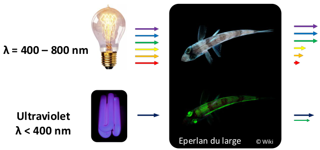
Figure 2 - Scheme representing linear (top) and nonlinear (bottom) optics. An Eperlan du large (middle picture) receives light at given wavelengths λ (left picture and colored arrow). The emitted light spectrum (right colored arrow) depends on the incident light. In linear optics, the fish receives visible wavelengths (400-900 nm) and reflects light with the same spectral components and different intensity. Here, the fish has absorbed red, orange, and yellow wavelengths, making it appear purple, blue and green. In nonlinear optics, the fish receives UV light (λ < 400 nm) and emits both reduced UV and green light; this phenomenon is fluorescence.

The energy shift, called the Stokes shift, can be important for fluorescence technique sensitivity [The Molecular Probes® Handbook—A Guide to Fluorescent Probes and Labeling Technologies]. Fluorescence encompasses these three stages, illustrated by Jablonski diagrams (Figure 3). The non-radiative transitions introduce a time delay between excitation and emission referred to as the excited state lifetime \(\tau\), which is typically measured to characterize a fluorophore.

Figure 3 - Jablonski diagram of absorbance, non-radiative decay, and fluorescence. Electronic transitions are about 1 eV. Absorption is about 1 femtosecond, relaxation takes about 1 picosecond, fluorescence takes about 1 nanosecond. S0 and S1 represent different electronic states. The other numbers (here 0–3 are shown) represent vibrational states. By Jacobkhed from the Jablonski Wikipedia page (French version).

All biological and most organic materials fluoresce when excited with UV light [Misra et al. 2025]. The intensity of fluorescence is not constant and depends on the physiological (i.e., physical and chemical) state [Gorbunov et Falkowski 2022] of the fluorescent material and its environment (pH, Cl⁻ concentration, temperature, CO₂ levels, etc.). In a fluorescent material, only a portion of the excited molecules produce fluorescence emission as other processes may also depopulate the excited state. Quenching refers to any process that decreases fluorescence intensity [Lakowicz 2006]. The ratio between the number of fluorescence photons emitted to the number of photons absorbed measures the fluorescence efficiency and is referred to as quantum yield. Learn more about fluorescence in [Nodin et al. 2014] (French) or in the Molecular Probes Handbook.

To summarize, the five key parameters in fluorescence are:

• The excitation spectrum and the maximal excitation wavelength

• The emission spectrum and the maximal emission wavelength

• The excited state lifetime: \(\tau\)

• The quantum yield

• Molar absorption coefficient: relates the absorbance to the molecular concentration using Beer-Lambert’s law

▶ Proxy applications

Fluorescence is exploited across multiple disciplines, from cancer detection to quality control in industrial processes. Fluorescence has led to two Nobel prizes: one for green fluorescent protein (GFP) applications and one in 2014 for high-resolution fluorescence microscopy. In oceanography, fluorescence is used as a proxy (statistics) for unobservable or immeasurable variables in biology, physics, and chemistry.

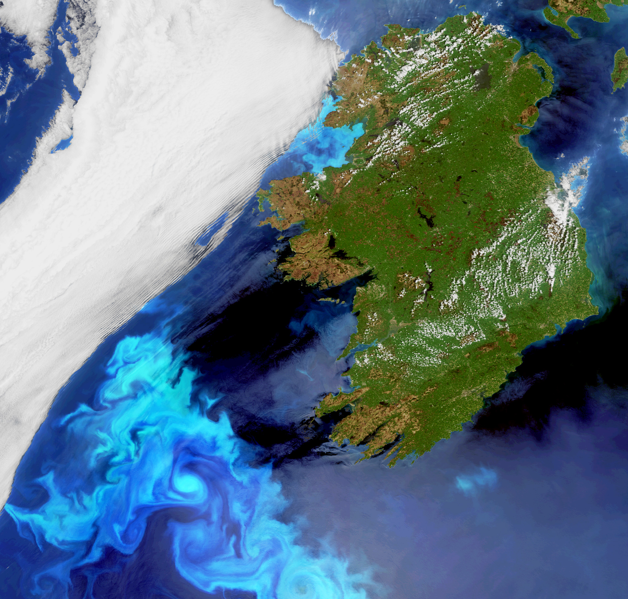
Figure 4 - Electric blue blooms off Ireland in the Envisat image - ©ESA - see this website for details.

Biological oceanography applications

• Biofluorescence serves important functions in marine ecosystems, with natural biofluorescence observed in fish, sharks, and other marine organisms. This natural fluorescence aids in species identification and behavioral studies [Gruber et al. 2016].

• Phytoplankton biomass is one of the essential ocean variables (EOV) that can be seen from space when they bloom (Figure 4) and can be studied with fluorimetry. Fluorescence is correlated with Chlorophyll-a, which is a proxy for phytoplankton biomass [Lorenzen 1966]. Different phytoplankton species exhibit distinct fluorescence signatures, enabling community structure analysis and species differentiation [Gorbunov et Falkowski 2022; Harris et al. 2024]. A comprehensive summary of fluorescence and chlorophyll-a and -b measurements is given in [Nodin et al. 2014].

• Coral fluorescence patterns serve as indicators of coral stress and health. Changes in fluorescence intensity and spectral characteristics can detect early signs of environmental stress before visible symptoms appear [Roth et Deheyn 2013].

Tracer and water mass studies

• Fluorescent dye tracing techniques are widely used in hydrology to map the motion of rivers and ocean currents with fluorometers [Wilson et al.]; [Park et al. 2023]. Their usefulness as water tracers is based on their visibility at low concentrations, fluorescent properties, cost, relationship to pH and salinity, photochemical decay, and resistance to absorption on mineral and organic surfaces. A comparison of eight fluorescent dyes was conducted by [Smart & Laidlaw 1977]. Fluorescein (green) and Rhodamine WT (orange) are preferred and can be combined.

• Non-marine objects, such as plastic debris (from micro to macro), oil spills, or human bodies, can be more easily tracked using fluorescent cameras and sensors than with visible light cameras [Misra et al. 2025].

Chemistry

• Dissolved organic matter (DOM) helps track biogeochemical processes, circulation patterns, and water masses. Colored dissolved organic matter (CDOM) is the subset of DOM that absorbs light over a broad range of visible and UV wavelengths and is a useful tracer for carbon and a proxy for mixing in various environments [Coble 2007]; [Gonçalves-Araujo et al., 2016]. Fluorescent DOM (fDOM) is a useful tracer for freshwater such as polar waters, and their distinct fluorescence spectra are even used to track their origin [Gonçalves-Araujo et al., 2016]. Note that fDOM is colored but not all CDOM is fluorescent [Coble 2007]. Open-source colorimeters using techniques other than fluorimetry exist [Anzalone et al. 2013].

Chemical sensing through quenching: Fluorescence intensity depends strongly on environmental parameters through quenching processes. These relationships are exploited in optodes for measuring:

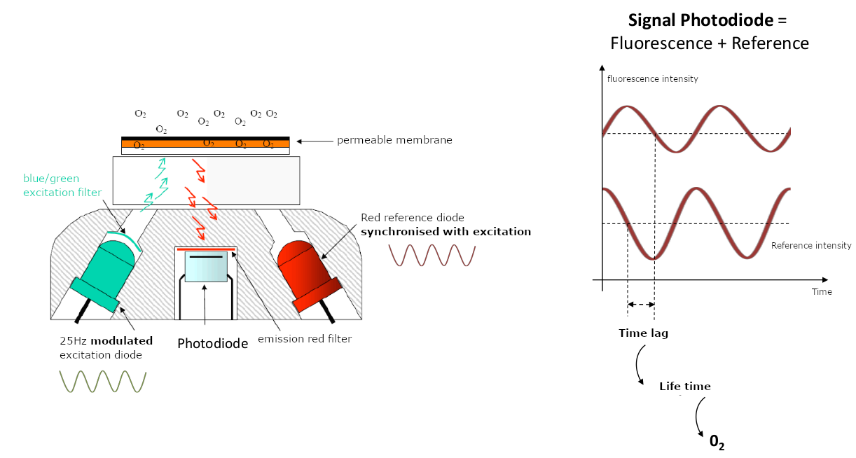
• Dissolved oxygen: Higher oxygen concentrations quench fluorescence intensity (see more in the oxygen section)

• pH monitoring: Fluorescent dyes sensitive to hydrogen ion concentration serve as proxies for pH measurements [Szapoczka et al. 2023]

The environmental sensitivity that initially appears as a limitation becomes an advantage when properly calibrated, enabling multi-parameter sensing with single fluorescent systems. Planar optodes are used to study O₂ and pH evolution through sediment to quantify bioturbation [Larsen et al. 2011]. Luminophores, i.e., colored sand grains visible under UV light, are also typically used in bioturbation studies [Mahaut & Graf 1987].

▶ Units and standards

When measuring light spectra, units can either be arbitrary units (AU) or fluorescence intensity. To measure a concentration, the units and calibration depend on the parameter of interest and become challenging when dealing with living organisms.

Instrument-specific calibration coefficients must account for temperature dependencies, non-linear response at high concentrations, and potential quenching effects. Regular verification using certified reference materials and inter-comparison exercises between instruments are essential practices to maintain measurement accuracy and facilitate integration of datasets across different platforms and temporal scales.

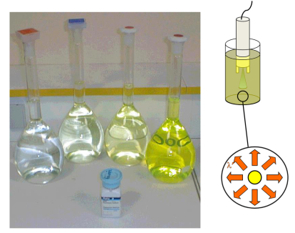
Figure 5 - (left) Five samples with different fluorescein concentrations used to calibrate a fluorometer. (right) Schematic diagram of a fluorometer calibration setup in a fluorescein solution that emits light at a given wavelength in all directions.

• For chlorophyll-a fluorescence measurements, primary calibration was performed using extracted chlorophyll solutions of known concentration, prepared from cultured phytoplankton or spinach extracts dissolved in acetone [Holm-Hansen et al., 1965; Lorenzen, 1966; Leeuw et al. 2013]. Today, standards mostly include stable fluorescent dyes such as Rhodamine WT [see the characteristics of a typical WiMo instrument] and Fluorescein (Figure 5). The results are expressed in μg/L or parts per billion (ppb). The conversion between fluorescence and chlorophyll involves corrections and assumptions; the final error can be constrained to about 30% see the 1st draft of Biogeochemical-Argo Implementation Plan.

• CDOM fluorescence is conventionally calibrated against quinine sulfate dihydrate solutions, with results expressed in Quinine Sulfate Units (QSU) or ppb quinine sulfate equivalents.

▶ References

Websites

• NKE instrumentation: https://nke-instrumentation.fr

• Thermofisher: https://www.thermofisher.com

Books and reports

• The Molecular Probes® Handbook—A Guide to Fluorescent Probes and Labeling Technologies: accessible on Thermofisher website

• Wilson, J. F.; Cobb, E. D.; Kilpatrick, F. A. Fluorometric Procedures for Dye Tracing.

Scientific publications

• Anzalone, G. C.; Glover, A. G.; Pearce, J. M. Open-Source Colorimeter. Sensors 2013, 13 (4), 5338–5346. doi.

• Gruber, D. F.; Loew, E. R.; Deheyn, D. D.; Akkaynak, D.; Gaffney, J. P.; Smith, W. L.; Davis, M. P.; Stern, J. H.; Pieribone, V. A.; Sparks, J. S. Biofluorescence in Catsharks (Scyliorhinidae): Fundamental Description and Relevance for Elasmobranch Visual Ecology. Sci Rep 2016, 6 (1), 24751. doi.

• Gorbunov, M. Y.; Falkowski, P. G. Using Chlorophyll Fluorescence to Determine the Fate of Photons Absorbed by Phytoplankton in the World’s Oceans. Annual Review of Marine Science 2022, 14 (Volume 14, 2022), 213–238. doi.

• Gonçalves-Araujo, R.; Granskog, M. A.; Bracher, A.; Azetsu-Scott, K.; Dodd, P. A.; Stedmon, C. A. Using Fluorescent Dissolved Organic Matter to Trace and Distinguish the Origin of Arctic Surface Waters. Sci Rep 2016, 6 (1), 33978. doi.

• Harris, P. D.; Ben Eliezer, N.; Keren, N.; Lerner, E. Phytoplankton Cell-States: Multiparameter Fluorescence Lifetime Flow-Based Monitoring Reveals Cellular Heterogeneity. The FEBS Journal 2024, 291 (18), 4125–4141. doi.

• Holm-Hansen, O., Lorenzen, C. J., Holmes, R. W., & Strickland, J. D. (1965). Fluorometric determination of chlorophyll. ICES Journal of Marine Science, 30(1), 3-15.

• Lorenzen, C. J. A Method for the Continuous Measurement of in Vivo Chlorophyll Concentration. Deep Sea Research and Oceanographic Abstracts 1966, 13 (2), 223–227. doi.

• Mahaut, M.-L.; Graf, G. A Luminophore Tracer Technique for Bioturbation Studies. Oceanologica Acta 1987.

• Misra, A. K.; Acosta‑Maeda, T. E.; Trimble, A. Z.; Zhou, J.; Liu, Y.-S.; Porter, J. N.; Egan, M. J. Standoff Real-Time Detection of Floating and Submerged Objects in Ocean Water. Sci Rep 2025, 15 (1), 31466. doi.

• Park, K. T.; Creelman, J. J.; Chua, A. S.; Chambers, T. S.; MacNeill, A. M.; Sieben, V. J. A Low-Cost Fluorometer Applied to the Gulf of Saint Lawrence Rhodamine Tracer Experiment. IEEE Sensors Journal 2023, 23 (15), 16772–16787. doi.

• Roth, M. S.; Deheyn, D. D. Effects of Cold Stress and Heat Stress on Coral Fluorescence in Reef-Building Corals. Sci Rep 2013, 3 (1), 1421. doi.

• Smart, P. L.; Laidlaw, I. M. S. An Evaluation of Some Fluorescent Dyes for Water Tracing. Water Resources Research 1977, 13 (1), 15–33. [doi]https://doi.org/10.1029/WR013i001p00015.

• Szapoczka, W. K.; Truskewycz, A. L.; Skodvin, T.; Holst, B.; Thomas, P. J. Fluorescence Intensity and Fluorescence Lifetime Measurements of Various Carbon Dots as a Function of pH. Sci Rep 2023, 13 (1), 10660. doi.

---

Sensing

Three main types of fluorimetry are used, each with distinct principles and applications in oceanographic instrumentation.

Fluorescence intensity change

Fluorescence intensity measurements are the most common approach for measuring chlorophyll-a and colored dissolved organic matter (CDOM) concentrations.

▶ Principle

Fluorescence intensity measurements rely on detecting the transmitted light intensity when a sample is excited at a specific wavelength. The basic principle follows the Beer-Lamber’s law :

\(I_f = K \cdot I_0 \cdot (1- e^{- \epsilon c L})\)

Where:

• \(I_f\) = fluorescence intensity

• \(K\) = quantum yield

• \(I_0\) = incident light intensity

• \(\epsilon\) = molar absorption coefficient

• \(c\) = fluorophore concentration

• \(L\) = path length

For low concentrations, fluorescence intensity is proportional to concentration. At high concentration the fluorescence intensity is no longer linear with the concentration.

Typical excitation and emission wavelength are:

• Chlorophyll-a: Excitation ~470 nm (blue), Emission ~690 nm (red). [Lorenzen 1966]; [Industrial].

• CDOM: Excitation ~350-380 nm (UV), Emission ~450-520 nm (blue-green). [Industrial].

The measurement geometry between emission and reception is typically at 90° to minimize interference from excitation light and scattered light (Figure 6). The most crucial elements in a fluorimeter are the excitation source and the detector. Additional filters are used to enhance signal-to-noise ratio, supress impact of scattering and potentially to decrease sensitivity to make measurement in high concentration (where the realtionship is not linear anymore) [Lorenzen 1966].

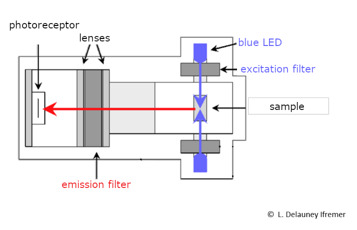
Figure 6 - Typical fluorometer geometry showing excitation light source, sample, and detector positioned at 90° angle

▶ Different types of sensors

Fluorometers are most commonly LED-based for their long lifetime and low power consumption.

Photodetector options:

• Photodiodes: Fast response, good sensitivity, most common choice [Leeuw et al. 2013]

• Photomultiplier tubes (PMTs): High sensitivity but require high voltage [Lorenzen 1966]

• Camera and smartphones detectors : Interesting for DIY but requires validation before hands [Friedrichs et al. 2017]

• Silicon detectors with filters: Cost-effective for specific wavelengths

▶ Typical characteristics

For chlorophyll-a fluorometers:

• Detection limit: 0.02-0.04 μg/L [Industrial; Lorenzen 1966] 0.10 μg/L [DIY SmartFluo project [Friedrichs 2017]]

• Dynamic range: 0-500 μg/L (Industrial) ; 0-250 μg/L (SmartFluo)

• Resolution: 0.03 μg/L (Industrial)

• Response time: <1 second (Both)

• Accuracy: ±5% or ±0.02 μg/L (whichever is greater)

For CDOM/fDOM fluorometers (Industrial):

• Detection limit: 0.1-1 ppb quinine sulfate units (QSU)

• Dynamic range: 0-150 QSU (CDOM); 0-1500 ppb QSU (fDOM)

• Resolution: 0.1 QSU

▶ Advantages and limitations

Advantages:

• Simple and robust measurement principle

• Fast response time suitable for real-time monitoring

• Wide dynamic range

• Low power consumption in LED-based designs

Limitations:

• Affected by temperature variations

• Subject to quenching effects (oxygen, pH, salinity)

• Fouling affects accuracy

• Cannot distinguish between different types of particles directly

• Requires regular cleaning and calibration

Fluorescence spectroscopy

Fluorescence spectroscopic measurements provide spectral information about fluorescent materials, enabling identification and differentiation of various fluorophores.

▶ Principle

A spectrofluorometer measures the emission spectrum of a sample, i.e., the intensity of emission over a broad range of wavelengths. It can also be used to determine the excitation spectrum when monitoring at a fixed emission wavelength. Compared to the fluorometer (which measures the intensity of only one wavelength), a spectrofluorometer provides a “fingerprint” of the fluorescent material (Figure 7).

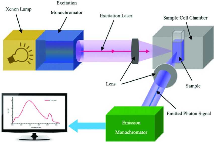
Figure 7 - Schematic diagram of the arrangement of optical components in a typical spectrofluorometer - from Spectrofluorometer Wikipedia page.

With this method one can work with Excitation-Emission Matrices (EEMs):

• Systematic measurement across multiple excitation and emission wavelengths

• Creates 3D plots showing fluorescence intensity as a function of both wavelengths

• Enables identification of multiple fluorophore components and quantifies their relative concentrations

Developments in data analysis techniques led to increased understanding of marine CDOM and improved algorithms for remote sensing correction [Coble 2007].

▶ Different types of sensors

The setup of a spectrofluorometer requires a source of excitation (light and filter or monochromator which can select a wavelength automatically and create an excitation beam), and an emission filter and measurement system (a photoreceptor and a filter or monochromator to measure the intensity of the different wavelengths one by one), within a black chamber (Figure 8). Contributions on this section are needed.

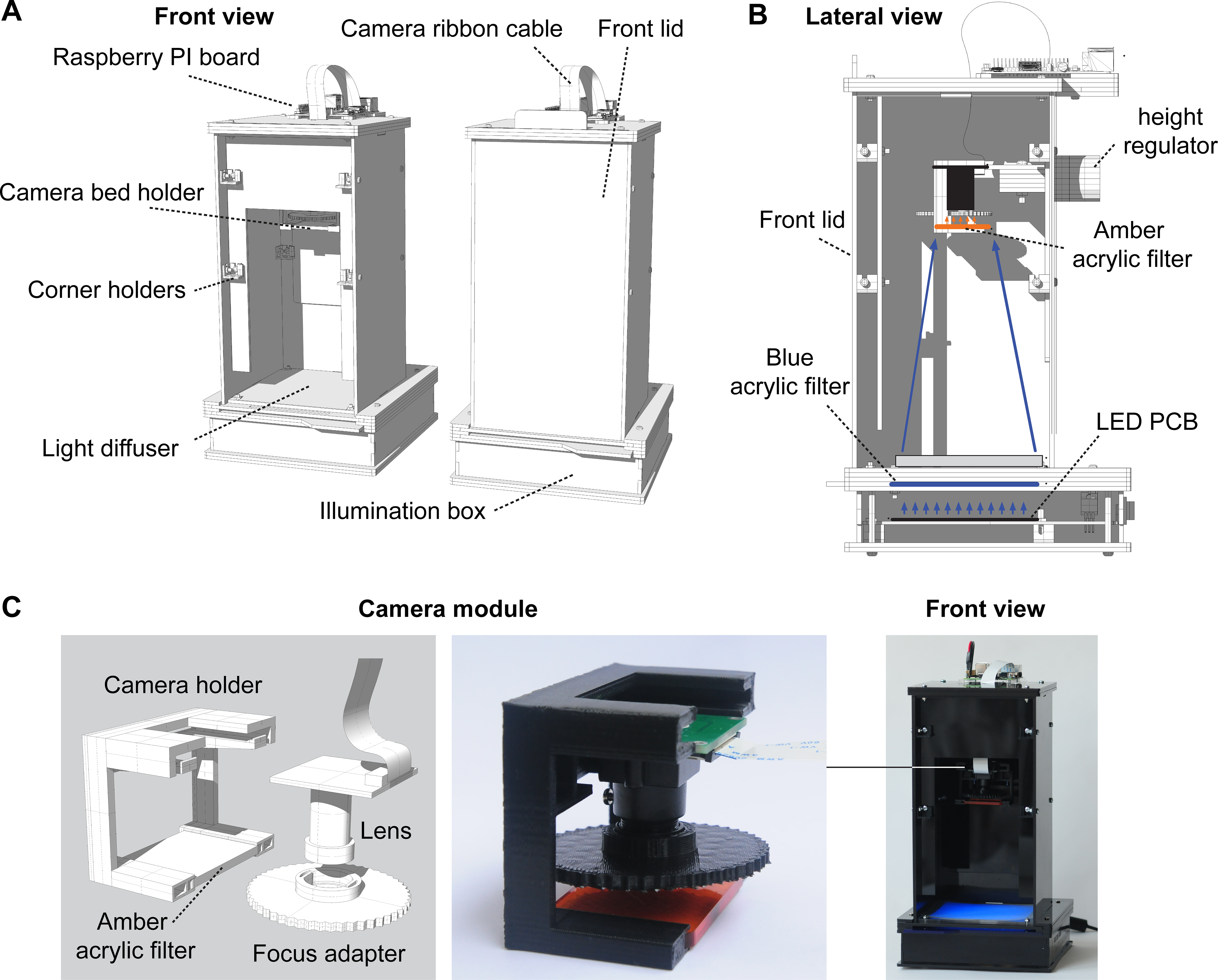
Figure 8 - (A) Schematic rendering of the device with and without the front lid. (B) Lateral view of a longitudinal cross-section of the device showing height control, illumination box and filters. (C) Camera and amber filter holder. From the open-source multifluorescence project FluoPi [Nuñez et al. 2017].

To learn more about fluorescence imaging system setup, have a look at the FluoPi DIY project [Nuñez et al. 2017] and the Basic Fluorescence Spectroscopy setup video.

▶ Typical characteristics

Multi-wavelength fluorometers:

• Size: 30-50 cm height, 3-8 kg

• Number of channels: 4-8 typical

• Excitation wavelengths: User-selectable LEDs

• Detection: Single PMT or photodiode

• Measurement time: 1-10 seconds per complete spectrum

▶ Advantages and limitations

Advantages:

• Multiple parameter measurement in single instrument

• Reduced interference from overlapping signals

• Better characterization of the spectrum

Limitations:

• Higher complexity and cost

• Longer measurement times

• Requires sophisticated data processing

• More sensitive to optical alignment

• Higher power consumption

• Complex calibration procedures

Fluorescence Lifetime Measurements

Fluorescence lifetime measurements detect the decay time of fluorescence emission, providing additional discrimination capability and reduced interference from scattered light.

▶ Principle

Fluorescence lifetime (τ) is the average time a molecule remains in the excited state before emitting a photon. It is typically used to measure O2 concentration (Figure9).

Figure 9 - by O.Fauvarque

▶ Different types of sensors

▶ Typical characteristics

▶ Advantages and limitations

References

▶ Publications

Fluorescence intensity methods:

• NKE, Aquared, RbR.

• Friedrichs, A.; Busch, J. A.; Van der Woerd, H. J.; Zielinski, O. SmartFluo: A Method and Affordable Adapter to Measure Chlorophyll a Fluorescence with Smartphones. Sensors 2017, 17 (4), 678. https://doi.org/10.3390/s17040678.

• Lorenzen, C. J. (1966). A method for the continuous measurement of in vivo chlorophyll concentration. Deep Sea Research and Oceanographic Abstracts, 13(2), 223-227. doi

• Holter, E., Hovkeer, K., & Zaneveld, J. R. V. (2003). Measurement of the absorption and attenuation of visible light by particles suspended in seawater. Limnology and Oceanography: Methods, 1, 1-13.

Fluorescence spectroscopy:

• Coble, P. G. Marine Optical Biogeochemistry:  The Chemistry of Ocean Color. Chem. Rev. 2007, 107 (2), 402–418. https://doi.org/10.1021/cr050350+.

• Murphy, K. R., Stedmon, C. A., Graeber, D., & Bro, R. (2013). Fluorescence spectroscopy and multi-way techniques. PARAFAC. Analytical Methods, 5(23), 6557-6566. doi

• Nodin, L.; Meallet-Renault, R.; Piard, J. Séparation et Étude Des Pigments Des Épinards Par Spectrofluorimétrie. Le Bulletin de l’Union des Professeurs de Physique et de Chimie 2014, 108 (961), 293–310.

Fluorescence lifetime:

• Sauer, M., Hofkens, J., & Enderlein, J. (2011). Handbook of Fluorescence Spectroscopy and Imaging: From Single Molecules to Ensembles. Wiley-VCH.

• Lakowicz, J. R. (2006). Principles of Fluorescence Spectroscopy. 3rd Edition, Springer. doi

DIY implementations:

• Leeuw, T., Boss, E., & Wright, D. L. (2013). In situ measurements of phytoplankton fluorescence using low cost electronics. Sensors, 13(6), 7872-7883. doi

• Friedrichs, A.; Busch, J. A.; Van der Woerd, H. J.; Zielinski, O. SmartFluo: A Method and Affordable Adapter to Measure Chlorophyll a Fluorescence with Smartphones. Sensors 2017, 17 (4), 678. https://doi.org/10.3390/s17040678.

• Nuñez, I.; Matute, T.; Herrera, R.; Keymer, J.; Marzullo, T.; Rudge, T.; Federici, F. Low Cost and Open Source Multi-Fluorescence Imaging System for Teaching and Research in Biology and Bioengineering. PLOS ONE 2017, 12 (11), e0187163. https://doi.org/10.1371/journal.pone.0187163.

---

Available sensors

📋 Interactive Table Features:
• Drag & Drop: Click and drag column headers to reorder columns
• Links: URLs are converted to clickable blue link (🔗) icons

Sensor name ⇄	technology ⇄	measured quantity ⇄	absolute accuracy ⇄	range ⇄	relative accuracy ⇄	stability ⇄	Validation level ⇄	Associated publication ⇄	Mecanic integration ⇄	electronic integration communication interface ⇄	Sampling volume ⇄	Max. depth ⇄	Cost ⇄	Datasheet link ⇄	Where to buy? ⇄	Excitation & Fluorescence wavelengths (nm) ⇄	Calibration fluorophore ⇄
Trilux	Optic	Chlorophyll a Phycerythrin/Phycocyanin Nephelometry	—	0-100µg/L	—	—	—	—	Connecteur Impulse MCIL-6-MS	RS232 / analogique (0-5V)	(diam) 26 mm x (long) 60mm	600m	2500 (2023)	🔗	🔗	N.C.	—
ECO FL	Optic	CHL-A	—	—	—	—	—	—	—	RS232	—	600m	9000 (2024)	🔗	🔗	470 / 695 nm	—
C3 / C6	Optic	CHL-A	—	0-500 µg/L	—	—	—	—	—	RS232	—	600m	—	🔗	🔗	—	—
Wimo (NKE)	Optic	Chlorophylle A Phycocyanine Phycoérythrine	0.03 ppb* 0.1 ppb* 0.1 ppb*	0-500 ppb* 0-4500 ppb* 0-750 ppb*	<1% <1% <1%	—	—	—	—	Mobdus RS232/RS485 Solution 3G/4G	—	250m	—	🔗	🔗	—	*Rhodamine
SmartFluo	quantification of the red light present in the image taken by the phone	Chlorophyll a	1 DN/s ≤ e ≤ 80 DN/s (plus d’erreur proche de 1 que de 80 DN/s)	Min : 10 µg/L Max : 250 µg/L	—	4-5 DN/s	—	—	—	—	—	Surface	33€ - 73 € + prix du smartphone	🔗	DIY	—	—
Fluoromètre Phytoplancton	quantification of the voltage transmitted after excitation of chlorophyll with a 448 nm LED	Chlorophyll a	e ≥ 0.3 µg/L	Min : 0 µg/L Max : 100 µg/L	4 % comparer à un instrument commercial	—	—	—	—	UART	—	2m	$ 150	🔗	DIY	448 nm	—
Chlorophyll-a HD DVD	quantification of the voltage transmitted after excitation of chlorophyll with the OPU laser at 405 nm	Chlorophyll a	0 µg/L ≤ e ≤ 4 µg/L	Min : 0.35 µg/L Max : 100 µg/L	< 4 %	—	—	—	—	UART	—	Surface	$ 140	🔗	DIY	405 nm	—
Fluoromètre Rhodomine	quantification of the voltage transmitted after excitation of the RWTs with a 555 nm LED	Rhodamine	0.11 mV ≤ e ≤ 0.37 mV	Min : 0.2 µg/L Max : 60 µg/L	2 %	—	—	—	—	—	—	500m	$ 750	🔗	DIY	555 nm	—

---

DIY projects specific to fluorescence

Sensor	EOV/EBV	Main Material	Classification	Scientific Article	Cost	Dissemination	Max Depth	Measurement Range	Measurement Error	Systematic Error	Comparison Sensor
SmartFluo: A Method and Affordable Adapter to Measure Chlorophyll a Fluorescence with Smartphones	Chlorophyll A	Smartphone	Open-source, Low cost	2017	30€ - 70€ + smartphone	Spain, Ireland, Germany, Norway	Surface	Min: 10µg/L - Max: 250µg/L	1DN/s < e < 80DN/s (DN: Digit number)	N/A	LS 55, PerkinElmer (R²= 0.98)
In situ Measurements of Phytoplankton Fluorescence Using Low Cost Electronics	Chlorophyll A	Arduino	Low cost	2013	150$$	United States (river)	2m	Min: 0.3µg/L - Max: 100µg/L	e ≥ 0.3µg/L	4% compared to commercial instrument	WETStar (R²= 0.886)
A low-cost and portable fluorometer based on an optical pick-up unit for chlorophyll-a detection	Chlorophyll A	Arduino, DVD Reader	Low cost	2023	140$$	N/A	Surface	Min: 0.35µg/L - Max: 100µg/L	e ≤ 4 µg/L	< 4%	N/A
A Low-Cost Fluorometer Applied to the Gulf of Saint Lawrence Rhodamine Tracer Experiment	Rhodamine	Custom PCB	Low cost	2023	750$$	Quebec	Surface	Min: 0.2µg/L - Max:60µg/L	0.11mV ≤ e ≤ 0.37mV	2%	Turner Cyclops-7 and AML X2Change (R²=0.99)
FluoPi: Low-cost multifluorescence imaging system	Multiple fluorophores	Raspberry Pi, Camera	Open-source, DIY	2017	~200$$	Global (online)	Benchtop	Variable (depends on filters)	Platform dependent	Platform dependent	Research-grade fluorometers
OpenCTD Fluorometer Extension	Chlorophyll A, CDOM	Arduino, OpenCTD platform	Open-source, Low cost	Ongoing	~100-300$$	Global (GitHub)	200m+	0-200µg/L (Chl-a)	~10%	Temperature dependent	Commercial CTD fluorometers
PhotosynQ: Handheld Photosynthesis Meter	Chlorophyll fluorescence	Custom hardware	Open-source, Educational	2015+	~500$$	Global (educational)	Surface/Laboratory	0.1-100 ΦPSII	~5%	Light dependent	PAM fluorometers