Oxygen#
The “Background” section summarizes typical characteristics of dissolved oxygen encountered in the ocean: oxygen concentration ranges, vertical profiles, and spatial and temporal scales. Oxygen measurements can be taken using “Sensing Technologies” including the Winkler method, electrochemical sensors (Clark-type electrodes) and optical sensors (fluorescence-based optodes).
Finally, a comprehensive table of sensors and instruments available on the market is provided in the “Sensors Database” section.
Contributions:
Background#
Dissolved oxygen is one of the main scalar used to characterized water masses in the ocean along with temperature and salinity. Its distribution is fundamental to aquatic ecosystem functioning and climate regulation. The ongoing increase in ocean deoxygenation due to global warming is of primary concern [Breitburg et al., 2018]. Best accuracy of dissolved oxygen were around \(8 \mu mol/kg\) in 2013 with scientific needs around \(1 \mu mol/kg\) to accurately oxygen cycle [Coppola et al. 2013].
You can measure dissolved oxygen to study numerous biogeochemical processes (photosynthesis, respiration, decomposition, solubility, circulation, mixing). Organisms ranging from unicellular to complex multicellular species depends on dissolved oxygene, from intertidal zones to deep oceans. Biogeochemical cycling of essential elements such as nitrogen and carbon depends on the dissolved oxygen cycle [Breitburg et al., 2018]. Spatial and temporal characterization of upwelling time and gyre widely use oxygene measurement as well as freshwater masses tracking and deep water reneawel in fjords [Emery and Thomson 1992].

Take a deep breath and dive into the oxygene cycle, discover typical spatial and temporal scales and its units and standards!
▶ Oxygen cycle: Production, consumption and minimum zones
Dissolved oxygen in the ocean is primarily produced through photosynthesis by phytoplankton (including cyanobacteria), algae, and to a lesser extent, seagrasses and kelp in coastal regions. Additional oxygen enters the ocean through gas exchange at the air-sea interface. Cold polar waters, which can hold higher concentrations of dissolved oxygen due to lower temperatures, sink and transport oxygen to deep ocean layers through thermohaline circulation (Figure 1).
Dissolved oxygen is consumed primarily through respiration by marine organisms and bacterial decomposition of organic matter. Oxygen is also lost through nitrification, photo-oxidation, or chemical oxidation, or transferred back to the atmosphere through air-sea gas exchange. Notably, approximately 50% of Earth’s atmospheric oxygen originates from oceanic photosynthesis.
This cycle is influenced by multiple factors including water temperature (which affects oxygen solubility), biological activity, oceanic circulation patterns at various scales, and atmosphere-ocean interaction processes such as sea state, wind speed, atmospheric pressure, relative humidity, and the CO₂ gradient between the atmosphere and ocean.
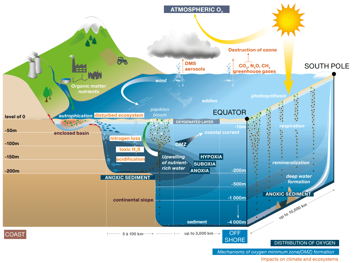
Figure 1 - Processes affecting O₂ dynamics in the ocean and mechanisms of oxygen minimum zones (OMZs) formation (figure from The Ocean revealed - chapter 8 [Paulmier, 2017]).#
Key definitions:
OMZs: Oxygen minimum zones are regions where a subsurface minimum oxygen level occurs. They are large, stable oceanic features pronounced in highly productive regions [Maas et al., 2014].
Oxycline: Zone of strong vertical oxygen gradient.
Hypoxia: Conditions of low oxygen concentration harmful to life, typically characterized by a 2 mg/L threshold (= 1.4 mL/L = 63 μmol/L). However, many organisms and ecological processes are affected at higher or lower oxygen concentrations.
Anoxia: The complete absence of oxygen.
▶ Spatial scales
A typical vertical oxygen profile presents a well-oxygenated layer near the surface (surface mixed layer), followed by a sharp decrease with depth referred to as the oxycline. At intermediate depths (200-1000m), oxygen minimum zones (OMZs) occur where respiration dominates (Figure 1 - 2). At greater depths (below 600m) water is well oxygenated [Maas et al., 2014; Alhassan et al., 2024].
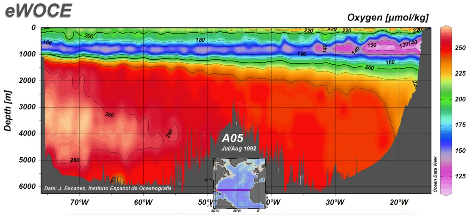
Figure 2 - Dissolved oxygen profile from a transect across the Atlantic Ocean from Florida to the coast of Africa (as in the inset). The oxygen minimum layer is visible between 500–1000 m. [By Alhassan et al. 2024 adapted from Garçon et al. 2019].#
Global Scale (1000-10000 km): Large-scale oxygen distribution patterns are controlled by thermohaline circulation (see oxygen cycle section). Major OMZs exist in the Eastern Tropical Pacific, Arabian Sea, and Bay of Bengal. The persistent OMZ of the Eastern Tropical Pacific spans hundreds of meters vertically and horizontally hundreds of kilometers, and lies just below the thermocline (Figure 2). In its core, OMZs can reach levels as low as 1 μM [Maas et al., 2014].
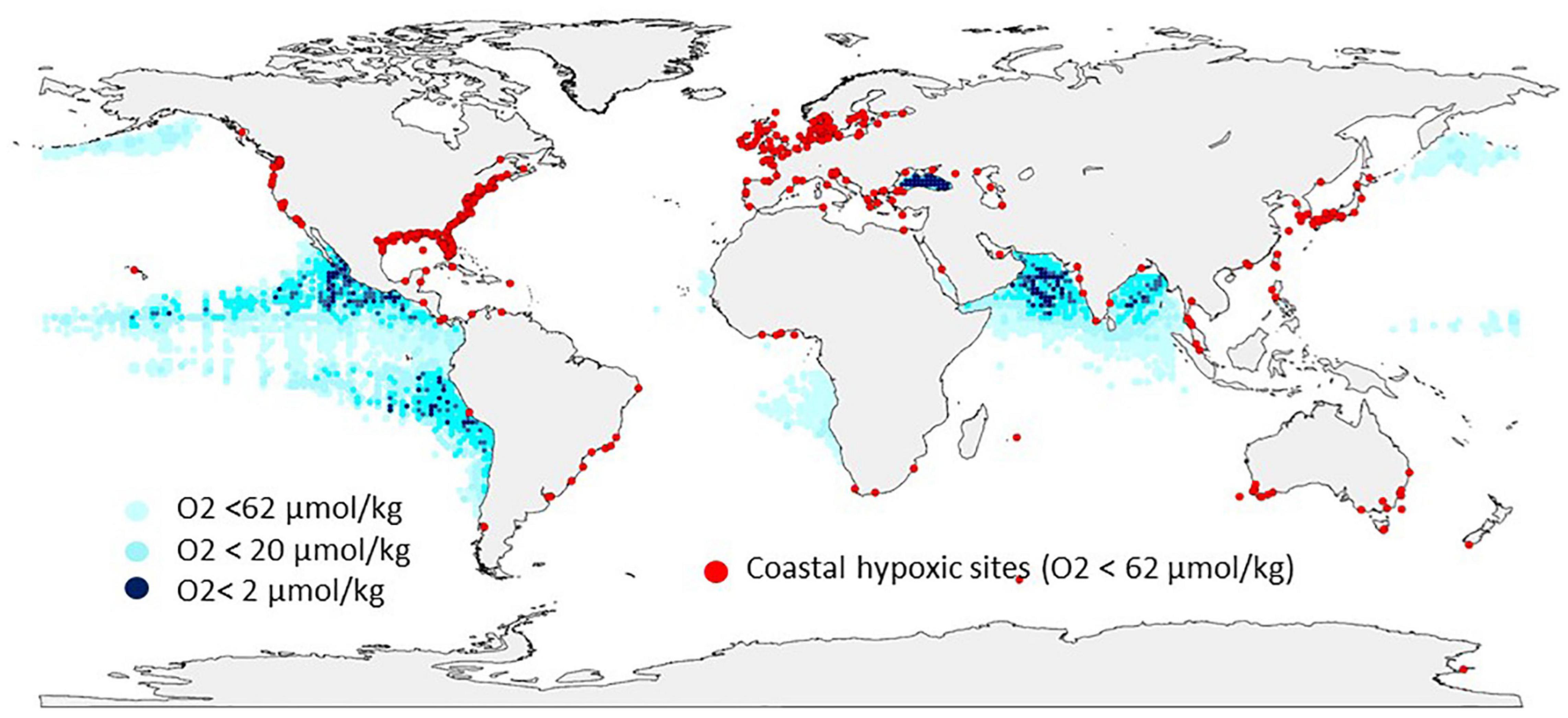
Figure 3 - Global distribution of low O₂ areas (i.e., \(O₂ < 62 \mu mol/kg\)) in the coastal and global ocean (from [Breitburg et al., 2018]). In coastal areas, more than 500 sites have been identified with low O₂ conditions in the past half century (red dots) while in the open ocean the extent of low O₂ waters amounts to several million km³ (the blue dots refer to conditions at 300 m). (Initially from [Breitburg et al. 2018 - UNESCO article]; [Grégoire et al., 2021]).#
Regional Scale (10-1000 km): Regional oxygen patterns are influenced by upwelling systems, continental margins, and regional circulation. Coastal upwelling brings oxygen-poor deep water to the surface (Figure 3).
Mesoscale (1-100 km): Eddies and fronts create oxygen fluctuations through vertical transport and biological productivity changes.
Local Scale (0.1-10 km): Fine-scale processes include benthic boundary layer dynamics, internal waves, and localized biological hotspots that create small-scale oxygen gradients. Areas with low oxygen levels, where hypoxia and anoxia occur, are localised natural phenomena that are specific to coastal environments. However, eutrophication is causing them to increase in size and number [Rabalais et al. 2014] (Figure 3).
Microscale (<1 km): Turbulent mixing, biogeochemical microenvironments, and organism-scale processes that affect local oxygen consumption and transport.
▶ Time series
Geological (>1000 years): Long-term climate variations affect global oxygen inventory and OMZ extent.
Centennial-Decadal (10-100 years): Climate change impacts on ocean deoxygenation, with observations showing 1-7% decrease (on the order of \(10^{15} mol\) in dissolved oxygen content for the complete water column) in global oxygen content since 1960 [Schmidtko et al., 2017; UNESCO GO2NE, 2018].
Interannual (1-10 years): Climate modes like El Niño/La Niña significantly affect oxygen distribution, particularly in tropical regions where OMZ intensity varies with climate oscillations.
Seasonal (months): Seasonal thermocline development affects stratification and oxygen vertical spreading. Spring blooms consume oxygen, while stormy weather mixing replenishes surface oxygen levels (Figure 4).
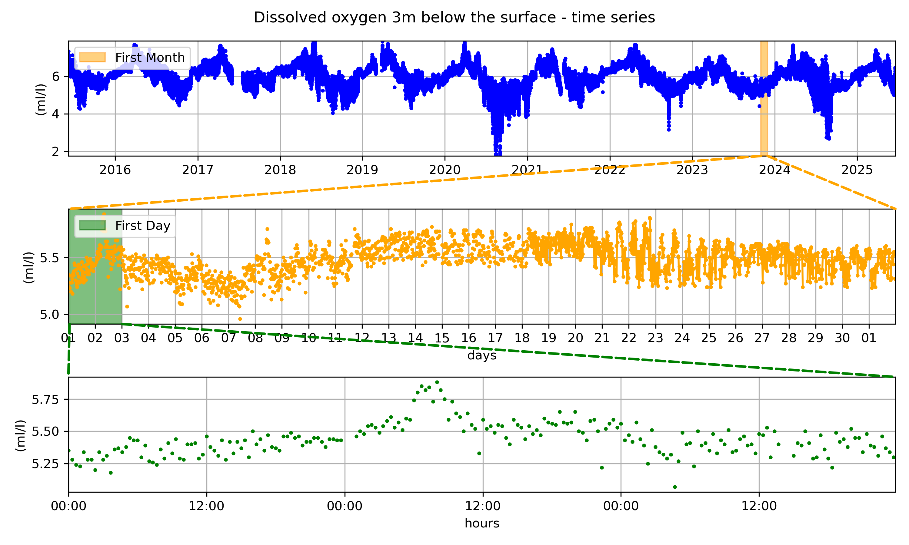
Figure 4 - COAST-HF-MAREL Iroise buoy dissolved oxygen measured 3 m below the surface at [48.35796°, -4.55175°] doi - by [Rimmelin-Maury et al.(2023)]. The complete data set can be viewed on the Coriolis website#
Daily-Weekly: Diel cycles driven by photosynthesis/respiration create daily oxygen fluctuations, particularly in productive coastal areas and coral reefs. Storms, here translated in a decrease in atmospheric pressure and increase in wind speed, may show local and punctual oxygen increase (Figure 5).
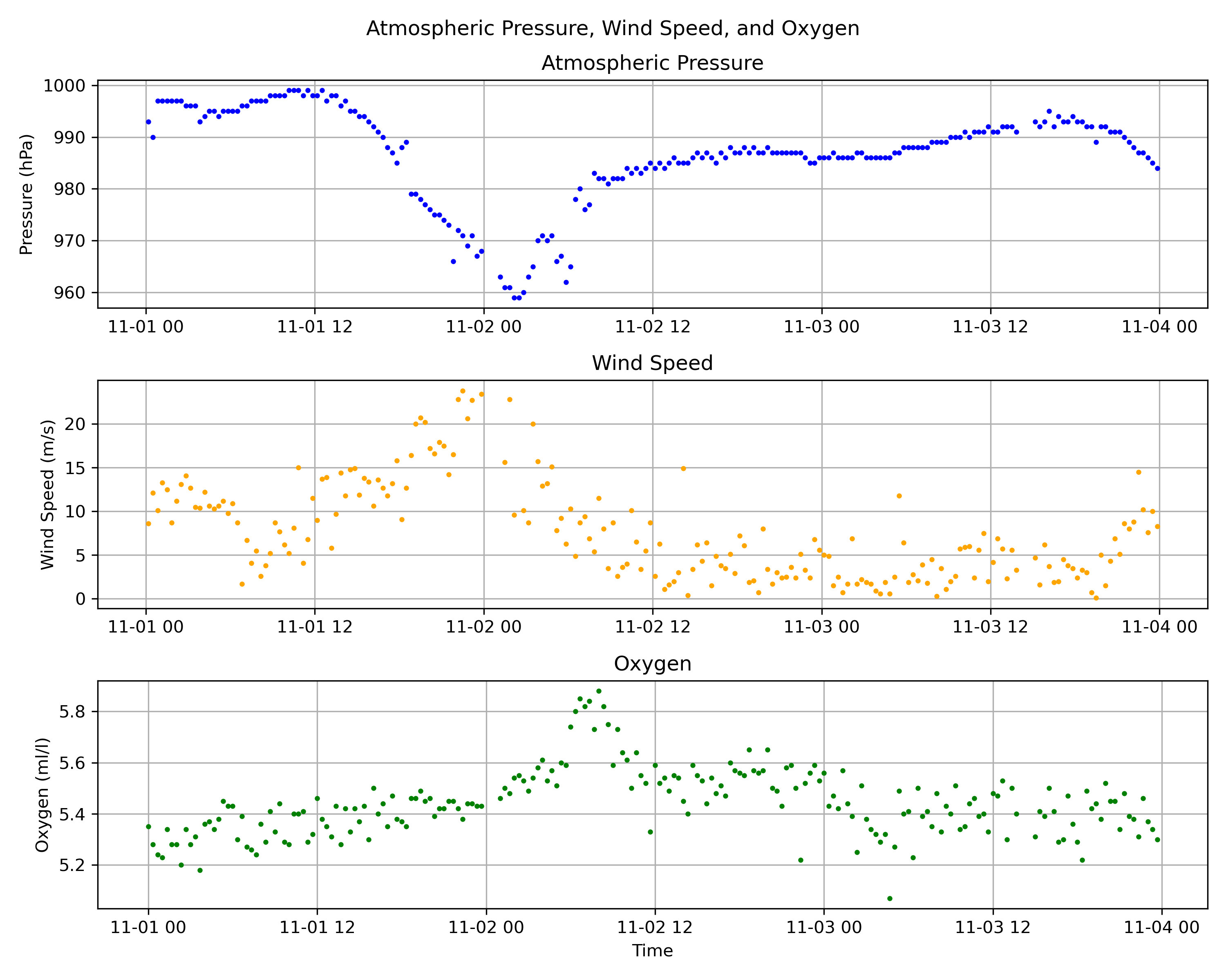
Figure 5 - Storm event observed from COAST-HF-MAREL Iroise buoy data set at [48.35796°, -4.55175°] doi - by [Rimmelin-Maury et al.(2023)]. The complete data set can be viewed on the Coriolis website#
High-frequency (<hours): Turbulent processes, internal waves, and rapid biological responses create short-term oxygen variability that requires high-resolution measurements.
▶ Standards, units and databases
Standard Units and Conversions
Dissolved oxygen concentrations can be expressed in several units, each with specific applications:
Primary concentration units:
μmol/kg (micromoles per kilogram): Gravimetric unit preferred for oceanographic research, where the value accounts for sample density variations [Bittig et al., 2015]
Volume-based units (related to oxygen molar volume and molar mass):
mg/L (milligrams per liter)
mL/L (milliliters per liter)
μmol/L (micromoles per liter)
Saturation units:
% saturation: Percentage of oxygen relative to equilibrium with atmosphere at given temperature, salinity, and pressure
Apparent Oxygen Utilization (AOU): Difference between saturation concentration and measured concentration (μmol/kg)
Conversion recommendations: See [Bittig et al., 2015] for detailed conversion protocols and best practices.
▶ Major Databases and Data Centers
Global databases:
World Ocean Database (WOD): NOAA’s comprehensive ocean data archive - https://www.ncei.noaa.gov/products/world-ocean-database
GLODAP: Global Ocean Data Analysis Project for biogeochemical parameters - https://www.glodap.info/
Argo: Global array of profiling floats with biogeochemical sensors - https://argo.ucsd.edu/
CCHDO: CLIVAR and Carbon Hydrographic Data Office - https://cchdo.ucsd.edu/
Regional databases:
SeaDataNet: European marine data infrastructure - https://www.seadatanet.org/
JAMSTEC: Japan Agency for Marine-Earth Science and Technology - https://www.jamstec.go.jp/e/
CSIRO: Australian Commonwealth Scientific and Industrial Research Organisation - https://www.csiro.au/
As noted by Gouretski et al. (2024): “The number of oxygen profile data from all instrument types within the World Ocean Database (Boyer et al., 2018) reached a total of more than 1.2 million by 2023. However, there are significant data quality issues in the historical oxygen database for many reasons, including instrumental errors, data collection failures, data processing errors, improper sample storage, and unit conversion errors.”
▶ References
Scientific publication
Alhassan, Y.; Siekmann, I.; Petrovskii, S. Mathematical Model of Oxygen Minimum Zones in the Vertical Distribution of Oxygen in the Ocean. Sci Rep 2024, 14 (1), 22248. doi.
Amy E. Maas, Sarah L. Frazar, Dawn M. Outram, Brad A. Seibel, Karen F. Wishner, Fine-scale vertical distribution of macroplankton and micronekton in the Eastern Tropical North Pacific in association with an oxygen minimum zone, Journal of Plankton Research, Volume 36, Issue 6, November/December 2014, Pages 1557–1575, doi.
Bittig, H. C.; Fiedler, B.; Fietzek, P.; Körtzinger, A. Pressure Response of Aanderaa and Sea-Bird Oxygen Optodes. Journal of Atmospheric and Oceanic Technology 2015, 32 (12), 2305–2317. doi.
Breitburg, D.; Marilaure, G.; Kirsten, I. The Ocean Is Losing Its Breath: Declining Oxygen in the World’s Ocean and Coastal Waters; Summary for Policy Makers; IOC. Technical series, 137; Document de programme de réunion IOC/2018/TS/137 REV; UNESCO, 2018. doi.
Garçon, V.; Karstensen, J.; Palacz, A.; Telszewski, M.; Aparco Lara, T.; Breitburg, D.; Chavez, F.; Coelho, P.; Cornejo-D’Ottone, M.; Santos, C.; Fiedler, B.; Gallo, N. D.; Grégoire, M.; Gutierrez, D.; Hernandez-Ayon, M.; Isensee, K.; Koslow, T.; Levin, L.; Marsac, F.; Maske, H.; Mbaye, B. C.; Montes, I.; Naqvi, W.; Pearlman, J.; Pinto, E.; Pitcher, G.; Pizarro, O.; Rose, K.; Shenoy, D.; Van der Plas, A.; Vito, M. R.; Weng, K. Multidisciplinary Observing in the World Ocean’s Oxygen Minimum Zone Regions: From Climate to Fish — The VOICE Initiative. Front. Mar. Sci. 2019, 6. doi.
Gouretski, V.; Cheng, L.; Du, J.; Xing, X.; Chai, F.; Tan, Z. A Consistent Ocean Oxygen Profile Dataset with New Quality Control and Bias Assessment. Earth System Science Data 2024, 16 (12), 5503–5530. doi
Grégoire, M.; Garçon, V.; Garcia, H.; Breitburg, D.; Isensee, K.; Oschlies, A.; Telszewski, M.; Barth, A.; Bittig, H. C.; Carstensen, J.; Carval, T.; Chai, F.; Chavez, F.; Conley, D.; Coppola, L.; Crowe, S.; Currie, K.; Dai, M.; Deflandre, B.; Dewitte, B.; Diaz, R.; Garcia-Robledo, E.; Gilbert, D.; Giorgetti, A.; Glud, R.; Gutierrez, D.; Hosoda, S.; Ishii, M.; Jacinto, G.; Langdon, C.; Lauvset, S. K.; Levin, L. A.; Limburg, K. E.; Mehrtens, H.; Montes, I.; Naqvi, W.; Paulmier, A.; Pfeil, B.; Pitcher, G.; Pouliquen, S.; Rabalais, N.; Rabouille, C.; Recape, V.; Roman, M.; Rose, K.; Rudnick, D.; Rummer, J.; Schmechtig, C.; Schmidtko, S.; Seibel, B.; Slomp, C.; Sumalia, U. R.; Tanhua, T.; Thierry, V.; Uchida, H.; Wanninkhof, R.; Yasuhara, M. A Global Ocean Oxygen Database and Atlas for Assessing and Predicting Deoxygenation and Ocean Health in the Open and Coastal Ocean. Front. Mar. Sci. 2021, 8. doi.
Paulmier, A., & Ruiz-Pino, D. (2009). Oxygen minimum zones (OMZs) in the modern ocean. Progress in Oceanography, 80(3-4), 113-128. DOI: 10.1016/j.pocean.2008.08.001
Rabalais, N.; Cai, W.-J.; Carstensen, J.; Conley, D.; Fry, B.; Hu, X.; Quiñones-Rivera, Z.; Rosenberg, R.; Slomp, C.; Turner, E.; Voss, M.; Wissel, B.; Zhang, J. Eutrophication-Driven Deoxygenation in the Coastal Ocean. oceanog 2014, 27 (1), 172–183. doi.
Schmidtko, S., Stramma, L., & Visbeck, M. (2017). Decline in global oceanic oxygen content during the past five decades. Nature, 542(7641), 335-339. DOI: 10.1038/nature21399
The Ocean Revealed; CNRS éditions: Paris, 2017.
Additional references
International programs and protocols:
UNESCO GO2NE Project (2018). The Ocean is Losing its Breath: Declining Oxygen in the World’s Ocean and Coastal Waters. IOC Technical Series, 137. https://unesdoc.unesco.org/ark:/48223/pf0000265196
Technical manuals and best practices:
Aanderaa Data Instruments. Oxygen Optodes: Best Practices, Calibration Information and Literature List. https://www.aanderaa.com/media/pdfs/aanderaa-oxygen-optodes-best-practices-calib-info-literature-list.pdf
GO-SHIP Program. Hydrographic Manual. http://www.go-ship.org/HydroMan.html
Ocean Best Practices Repository. https://repository.oceanbestpractices.org/
Uchida, H. CTDO2 processing procedures. GO-SHIP Manual. http://www.go-ship.org/Manual/Uchida_CTDO2proc.pdf
YSI Inc. Dissolved Oxygen Handbook: A Guide to Dissolved Oxygen Measurement. Ocean Best Practices Repository. https://repository.oceanbestpractices.org/bitstream/handle/11329/923/ysi_do_handbook.pdf
Sensing Technologies#
The three major methods to measure dissolved oxygen in seawater are: water bottle sampling with iodometric titration (Winkler method), electrochemical sensors, and optical sensors.
For a deeper discussion on dissolved oxygen measurements, comparisons and bias, see [Coppola et al. 2013] and [Gouretski et al. 2024].
Water sampling (Winkler titration)#
▶ Principle
Water is sampled at a given location and depth in the ocean. The oxygen in the sample is fixed using a manganese solution. The sample settles for 10-20 min and is stored in a dark room. It can be titrated within 12 h. The oxygen concentration is measured through either titration or spectrophotometric analysis (Figure 6).
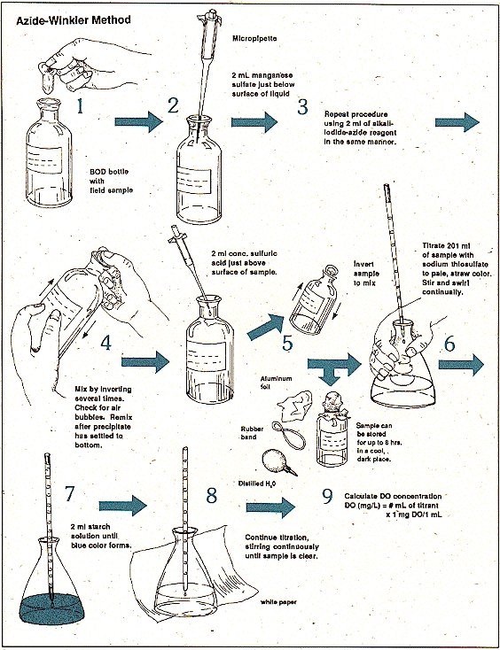
Figure 6 - Schematic of the Azide-Winkler method - © Washington State Department of Ecology.#
Educational resources on the Winkler method are available on the University of Montana website.
▶ Typical caracteristics
Accuracy : 1% (~2 \mu mpl/kg), provided the chemical analysis methods are rigorously applied [section 1.11.1.2 Emery and Thomson 1992]
Time response : ~30-60 min per sample
Sensitivity : -
Scale : Depends on the sampling strategy
▶ Advantages and limitations
Advantages:
Highest accuracy and precision available
Well-established reference method with decades of validation
Used as the gold standard for calibrating other methods
Independent of pressure, temperature, and salinity effects on sensors
Limitations:
No continuous measurements possible
Sample must be chemically “fixed” immediately → heavy procedure
Risk of sample contamination from ambient air
Photochemical oxidation if exposed to sunlight
Susceptible to errors from poor sampling procedures (e.g., inadequate bottle rinsing)
Operator dependent compared to other techniques
Electrochemical dissolved oxygen sensors (Clark cell)#
▶ Principle
The sensor measures changes in electric current resulting from the electrochemical reduction of oxygen at the cathode. Electrons transferred during this reduction generate a measurable current that flows through the electrolyte between the cathode and anode (Figure 7). The cathode is isolated from the surrounding medium by the electrolyte and an oxygen-permeable membrane, which minimizes the device’s sensitivity to turbulent flow fluctuations. The current produced is directly proportional to the oxygen concentration in the medium.
The sensor geometry affects the sensor signal: time response and stirring sensitivity depend on the length of the electrodes and the size of the sensitive tip - see more in section 3.1 [Revsbech 2021].
The main limitation of this method is that the cell must be recalibrated every several hours due to membrane fouling, chemical changes in the electrolyte [Coppola et al. 2013], and changes in the electrode surface properties [Emery and Thomson 1992].
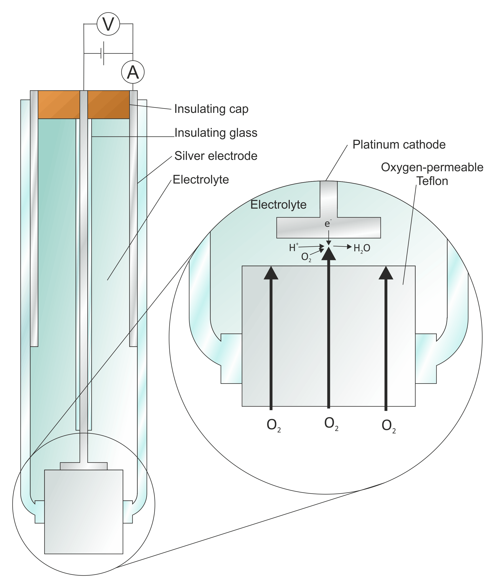
Figure 7 - A schematic representation of Clark’s 1962 invention, the oxygen electrode - by Larry O’Connell from the Clark electrode English Wikipedia page.#
▶ Typical characteristics
These values are based on the SBE43 Sea-Bird Electronics sensor [Coppola et al. 2013] and the review of micro-Clark sensors by [Revsbech 2021]:
Initial accuracy: ±2%
Time response: τ₆₃ < 1 s for the SBE43 and t₉₀ < 0.2 s [Revsbech 2021]
Resolution: 1 μmol/kg
Stability: Calibration drift rate of <2% over 1000 hours if kept clean
Size: Tip diameter < 2 μm for micro-Clark sensors [Revsbech 2021]
▶ Advantages and limitations
Advantages:
Very fast response time
Continuous real-time measurements
Good resolution
Proven technology for CTD integration
Limitations:
Requires frequent recalibration (every few hours to days)
Membrane replacement needed periodically
Sensitive to biofouling and contamination
Electrolyte consumption over time
Flow-dependent response
Not readily accessible for DIY applications
Clark-type electrodes were the first sensors used on biogeochemical Argo profiling floats, but have largely been replaced by optical sensors due to stability issues (more about the evolution of oxygen sensors on Argo floats in the introduction of [Gouretski et al. 2024]).
Optical Sensors (Optodes)#
▶ Principle
Optical oxygen sensors measure the quantity of light emitted by fluorescence from an oxygen-sensitive sensing foil (Figure 8). A blue LED excites luminescent compounds embedded in the sensing foil. The emitted light is at a different wavelength than the blue LED excitation light (see more on fluorescence in the fluorescence section). The emitted light is measured by a photodiode equipped with an optical filter. A red LED is used as a reference.
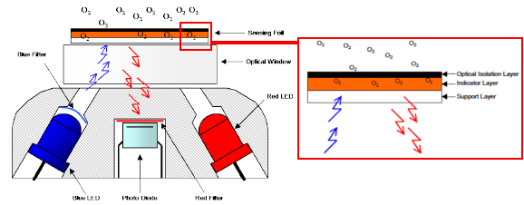
Figure 8 - Schematic of an optode sensor#
The foil is composed of three layers: the first layer provides optical isolation and is gas-permeable; the second layer is coated with a luminophore (fluorescent material such as platinum porphyrin complex), which is sensitive to oxygen; the third layer is a protective coating (Figure 8).
In the presence of oxygen, energy is transferred from the excited luminophore to the oxygen molecule through a process called dynamic quenching (Figure 9). This quenches the luminescence, reducing both the intensity and lifetime of the emitted light . The higher the oxygen concentration, the weaker the signal and the shorter the phase shift between the lifetime of the emitted light with O₂ versus without O₂ measured by the photodiode.
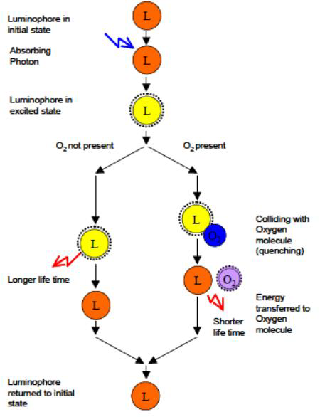
Figure 9 - Quenching reaction of a luminophore by oxygen#
The relationship between luminescence decay time and oxygen concentration follows the Stern-Volmer equation:
where \(\tau_0\) is the luminescence decay time in the absence of oxygen, \(\tau\) is the decay time with oxygen, \(K_{SV}\) is the Stern-Volmer constant, and \([O_2]\) is the oxygen concentration in \(\mu mol /L\).
Note that in a lifetime-based measurement, phase-shift is detected instead of decay time (see more in GO-SHIP manual - Uchida et al. 2010). The blue LED excite the luminophore with sinusoidally modulated intensity and emits a red luminescent light. The phase shift between the excited and emitted signals is function of the oxygen concentration.
▶ Typical characteristics
Initial accuracy: ±1% (or less) for optodes used on Argo floats [Claustre et al. 2020]
Time response: Manufacturer specifications [0.4-25 s] - Field tested [2-100 s]. Response time is sensitive to flow conditions (speed and temperature). Faster response times observed in pumped setups than in profilers or floats [Bittig et al. 2015]
Resolution: -
Stability: Stable over months to years - can auto-calibrate using atmospheric oxygen
Calibration: International recommendation for optodes calibration are given in the GO-SHIP manual - Uchida et al. 2010. Calibration over 3 points which include 0% and 100% oxygene saturation is recommanded as well as compison to Winkler measurements.
Compensation : Formulation to compensate salinity, temperature or depth effects may exist and be used in instrument ready to buy. They may not be explicited by the constructor.
▶ Advantages and limitations
Advantages:
Long-term stability (months to years)
Less sensitive to biofouling than electrochemical sensors
Lower power consumption
High precision
Pressure independent (no membrane compression effects)
Minimal stirring sensitivity
Easier calibration than other methods: optodes respond to pO₂ in both water and air with no bias [Claustre et al. 2020]
No electrolyte consumption (non-consuming measurement)
Limitations:
Slower response time than Clark-type sensors
Potential photobleaching of indicator dye over extended use
Temperature sensitivity requires careful compensation
Possible calibration drift in extreme conditions
Method Comparison#
Method |
Accuracy |
Response Time |
Stability |
Best Use |
|---|---|---|---|---|
Winkler |
±1% |
30-60 min |
Perfect |
Reference/calibration |
Clark electrode |
±2% |
<1 s |
Days-weeks |
Fast response applications |
Optical (optode) |
±1% |
2-100 s |
Months-years |
Autonomous deployments |
▶ References
Bittig, H. C.; Fiedler, B.; Fietzek, P.; Körtzinger, A. Pressure Response of Aanderaa and Sea-Bird Oxygen Optodes. Journal of Atmospheric and Oceanic Technology 2015, 32 (12), 2305–2317. doi.
Claustre, H.; Johnson, K. S.; Takeshita, Y. Observing the Global Ocean with Biogeochemical-Argo. Annual Review of Marine Science 2020, 12 (Volume 12, 2020), 23–48. https://doi.org/10.1146/annurev-marine-010419-010956.
Coppola, L.; Salvetat, F.; Delauney, L. et al (2013) White paper on dissolved oxygen measurements: scientific needs and sensors accuracy. Brest, France, IFREMER for JERICO, 22pp. DOI: http://dx.doi.org/10.25607/OBP-1022
Gouretski, V.; Cheng, L.; Du, J.; Xing, X.; Chai, F.; Tan, Z. A Consistent Ocean Oxygen Profile Dataset with New Quality Control and Bias Assessment. Earth System Science Data 2024, 16 (12), 5503–5530. https://doi.org/10.5194/essd-16-5503-2024.
Revsbech, N. P. Simple Sensors That Work in Diverse Natural Environments: The Micro-Clark Sensor and Biosensor Family. Sensors and Actuators B: Chemical 2021, 329, 129168. https://doi.org/10.1016/j.snb.2020.129168.
Uchida, H. CTDO2 processing procedures. GO-SHIP Manual. http://www.go-ship.org/Manual/Uchida_CTDO2proc.pdf
High-technology sensing and emerging techniques#
Sensors Database#
There is currently no database for the available oxygen sensors. Contributions are welcome, either follow the contribution guides or directly send a .csv table to diyoceano.bzh@listes.ifremer.fr