Turbidity#
The “Background” section summarises typical characteristics of turbidity encountered in estuaries and the open ocean : the range, vertical profile, and spatial and temporal scales encountered. Turbidity measurements can be acquired “Optically” (using sensors such as transmissiometers or nephelometers) or “Acoustically” (from backscatter of acoustic doppler current profiler (ADCP)).
Additional online ressources about the “art” of measuring turbidity can be found on the turbidity website.
Contributions:
Matthias Jacquet, Adèle Moncuquet
Background#

You can measure turbidity for a variety of purposes, such as determining the reduction in water visibility or quantifying the mass of suspended particle. Use this section to discover what is “turbidity” and how it’s typically used. Discover typical variations of turbidity depending on location, height above sea floor and time. Once you set your interest you can sneak a peak to the world of turbidity standard and units! Clearly define your environment and let’s dig into turbidity measurements.
▶ Introduction
Turbidity is a physical property of fluids that translates into reduced optical transparency, cloudiness, or haziness due to the presence of suspended material that modulates the transmission of light [Matos et al. 2024]. Turbidity is measured in three main ways: optically, acoustically with backscatter sensors, and remotely (satellite, aerial imaging).
Turbidity is a crucial measurement for the assessment of wastewater treatment, drinking water quality, aquaculture [Kitchener et al. 2017] and understanding coastal ecosystems [Bilotta & Brazier 2008]. In deep water, turbidity measurements is used to study deep mining impacts [Peacock & Alford 2018];[Munoz-Royo et al. 2022] and terrestrial mass transfer in canyons through turbidity currents [Khripounoff et al. 2003].
The link between turbidity and suspended sediment concentration (SSC) is site-dependent and requires careful calibration [Kitchener et al. 2017]. The characteristics of the sediment (shape, composition, etc.) vary depending on the environment and the meteorological and oceanographic conditions. Turbidity measurement is highly sensitive to suspended material type, particle shape, and particle size distribution. Therefore, turbidity measurement is site- and time-dependent. Combined measurements are typically used to obtain accurate suspended particulate matter (SPM) concentrations [Verney et al. 2024].
▶ Suspended materials
Seawater is composed of organic and inorganic matter with sizes ranging from molecular scale (< 1 nanometer) to centimeters (Figure 1 & 2). Suspended particulate matter measured as turbidity is organic and inorganic with size above 0.1 μm. Small particles (below 0.1 μm) can affect turbidity even if they are not SPM! For example, dissolved organic matter can affect the colour of the water, thereby modifying the turbidity without an increase in suspended particles [Anderson (2005)]. Turbidity is typically used to study sediments, which are inorganic particles. Distinguishing the different particles in turbidity measurements is a difficult task and combined measurements (particle sizer and multispectral sensors) are usually needed.
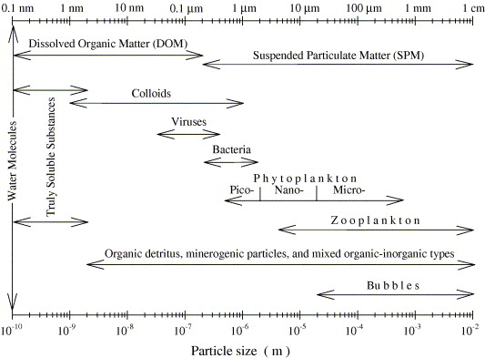
Figure 1 - Schematic diagram showing various seawater constituents in the broad size range from molecular size of the order of \(10^{−10}\) m to large particles and bubbles of the order of \(10^{−3}–10^{−2}\) m in size. The arrow ends generally indicate approximate rather than sharp boundaries for different constituent categories. Turbidity is used to quantify SPM but DOM may also affect turbidity measurement without an increase in suspended particles. From [Stramski et al. 2004]#
Organic and inorganic turbidity
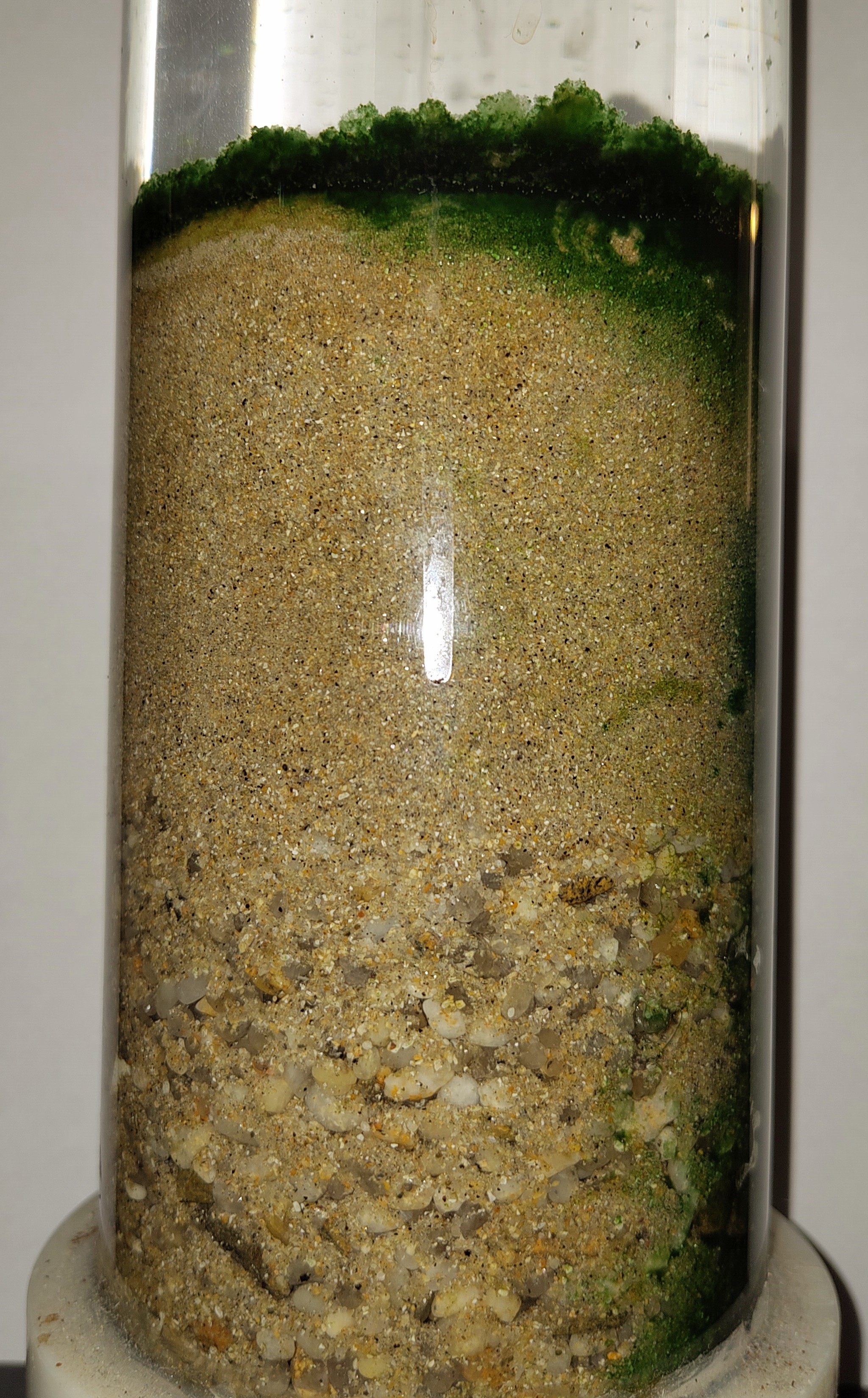
Figure 2 - Sedimentation column in the DHYSED laboratory#
Sediment
Sedimentary particles contribute significantly to turbidity measurements. These include various sediment sizes (ranging from clay particles <2 μm to sand particles >63 μm), different shapes (angular, rounded, elongated), densities (typically 2.5-2.7 g/cm³ for quartz), and compositions (quartz, feldspar, clay minerals, carbonates). Small inorganic matter is the dominant (submicrometer) contributors to light backscattering in open ocean conditions (outside of blooms) [Stramski et al. 2004]. Non-cohesive suspended sediments are well measured with acoustic backscatter, but cohesive sediments may not be well measured [Thorpe & Hanes 2002].
Organic
Organic material also contribute to turbidity measurements. This includes phytoplankton (algae and other microscopic organisms), detritus (decomposing organic matter), and bacterial biomass. Organic particles can have different optical properties compared to inorganic sediments, often absorbing specific wavelengths of light and contributing to both scattering and absorption signals [Matos et al. 2024]. Methods using optical measurements with different wavelengths are developed to differentiate inorganic from organic materials [Matos et al. 2019]. Acoustic backscatter can be dominated by phytoplankton with sufficiently high concentrations or during blooms [Stramski et al. 2004].
Other materials
Bubbles typically contaminate backscattered signals [Thorne & Hanes 2002]. Microplastics (particles <5 mm) are an emerging concern in turbidity measurements (Figure 3). These synthetic particles can interfere with traditional turbidity sensors as they have different optical properties than natural sediments. Their presence can lead to overestimation or underestimation of natural suspended sediment concentrations, depending on the measurement technique and particle characteristics.

Figure 3 - (left) Microplastics on the surface of water. (middle) Discarded plastic bag drifting over coral reef in current underwater. (right) Close up side shop of microplastics in someone’s hand. from NOAA website#
The use of measurements with distinctly different frequencies can allow distinguishing large (organic) particles from small (inorganic) particles, either in the case of acoustic sensing [Jourdin 2014] or optical sensing [Matos et al. 2024]. Finally, one has to keep in mind that comparison between turbidity measurements is almost impossible because particles (size, cohesive or non-cohesive) vary from site to site and directly affect turbidity.
▶ The diversity of environments
Turbidity intensity and patterns are variable along the land-sea continuum (Figure 2). Typical turbidity ranges vary from <1 NTU to >1000 NTU during highly productive events [Fondriest Environmental, Inc.]. Highly productive events depend on the environment and can produce saturation in turbidity measurements which become unusable.
In rivers, turbidity increase is naturally driven by heavy rains, snowmelt, ice scour or windstorms and present a seasonal cycle. High turbidity in rivers is also caused by human activity [Fondriest Envrionmental, Inc.]. Estuarine and coastal environments exhibit complex turbidity patterns and time variation. Tidal cycles, wind-driven resuspension, extreme events and seasonal variations in river discharge create dynamic turbidity patterns that require continuous monitoring [Verney et al. 2024].
In the deep ocean fresh sediment deposits are exceptional, which makes impacts from industrial activities long-lasting [Peacock & Alford 2018] and challenging due to the high pressure and low concentration (few mg/L)[Munoz-Royo 2022] and the need for long lasting measurements and reduced energy [Jiang et al 2020]. Natural sediment inputs are typically from turbidity currents triggered by earthquakes, storms, or river flooding [Bigham et al. 2021] or hydrothermal discharge. We welcome contributions on references relating to hydrothermal discharge.
Therefore, even at one site, turbidity will be driven by various forcing that can bring different types of particles. The clearer the knowledge on site forcings and associated particle flux the more accurate measurements are.
Figure 4 - The Bangladesh coastline seen by Envisat. The further from the coast, the darker the water color - ©ESA#
▶ Vertical profile
While vertical sediment concentration profiles (and flux) have been adequately determined for steady-state river flows, the response of these profiles and sediment fluxes to temporal or spatial flow changes remains largely unknown [Claudin et al. 2011].
However typical characteristics can be drawn : Turbidity typically decreases with depth in most environments. Surface waters often show higher turbidity due to wind mixing, phytoplankton blooms, and terrestrial inputs. A typical profile shows maximum values near the surface or bottom (due to resuspension), with a clear water layer in between. In stratified waters, the thermocline often coincides with a turbidity maximum due to particle accumulation at density boundaries.
▶ Time series
Turbidity exhibits variability across multiple temporal scales typically in relation to streamflow (Figure 5):
Tidal cycles: Semi-diurnal variations in coastal areas due to tidal resuspension
Daily cycles: Diurnal patterns driven by wind, temperature, and biological activity
Seasonal patterns: Related to river discharge, storm frequency, and biological productivity
Event-driven changes: Storms, floods, and anthropogenic activities cause rapid turbidity spikes
Long-term trends: Climate change and land-use modifications affect baseline turbidity levels
When deployed over a long period of time, biofouling is one of the main restriction for turbidity measurements. Constructors typically add automatic brushes to the instruments.
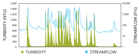
Figure 5 - Stream flow and turbidity are often directly related; as water flow increases, so will turbidity levels. From Fondriest Environmental, Inc.#
▶ Units and standards
Units and standards are a difficult aspect of turbidity. Several units are used and differ between US and EU standards. Also the method to calibrate instruments vary. Therefore two instruments calibrated under US and EU norms will give different results but with the same unit! Therefore it is important to state which standard was used during a tubidity measurement.
Units
Several units are used which depends on the measurement (Figure 6). A synthesis on turbidity units can be found in [Kitchener 2018].
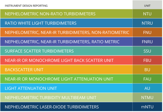
Figure 6 - The turbidity units used should be based on instrument design to ensure accurate and comparable data. From section Quality standard in Fondriest Environmental, Inc.#
The most common units are :
NTU (Nephelometric Turbidity Units): Optic unit. Most common, based on 90° light scattering : careful with the standard used (see below)
FAU (Formazin Attenuation Units) : Optic unit. Based on 180° light attenuation.
** dB (decibel) or BU** : Acoustic unit. Sound attenuation.
Standards
Several design standards are used to verify a turbidity meter and turbidity sensor performance. The method varies depending on the country, instrument design and the turbidity level.
Each methods consist on the measurement of the attenuation of a light source due to a concentration of formazin or other similar polymer-based calibration standard. The method differs on : the wavelength of the light source; the type of photo-detector, its position with respect to the light source and its distance to the sample.
The two main standards for optical measurements are :
NF EN ISO 7027-1:2016 recognizes two methods to measure turbidity in high and low turbidity conditions. Method accessible here and explicitely described in [Jacquet 2024].
USEPA Method 180.1 : main method used in USA [O’Dell 1996]. Note that eight standards are approved in USA for monitoring drinking water. More on turbidity standard on the Fondriest Website section quality standards.
Note that both methods can use NTU units but will give different values! One sample coud give 5.4 NTU with a USEPA 180.1 isntrument and 4.8 NTU with a ISO 7027 instrument! Today, in 2025, the definition of a standard for turbidity measurement is an ongoing process [Kitchener et al. 2017].
▶ References
Papers
Bilotta, G. S.; Brazier, R. E. Understanding the Influence of Suspended Solids on Water Quality and Aquatic Biota. Water Res 2008, 42 (12), 2849–2861. [doi]https://doi.org/10.1016/j.watres.2008.03.018.
Bigham, K. T.; Rowden, A. A.; Leduc, D.; Bowden, D. A. Review and Syntheses: Impacts of Turbidity Flows on Deep-Sea Benthic Communities. Biogeosciences 2021, 18 (5), 1893–1908. doi
Claudin, P.; Charru, F.; Andreotti, B. Transport Relaxation Time and Length Scales in Turbulent Suspensions. J. Fluid Mech. 2011, 671, 491–506. doi -Jiang, H.; Hu, Y.; Yang, H.; Wang, Y.; Ye, S. A Highly Sensitive Deep-Sea In-Situ Turbidity Sensor With Spectrum Optimization Modulation-Demodulation Method. IEEE Sensors Journal 2020, 20 (12), 6441–6449. doi
Jourdin, F.; Tessier, C.; Le Hir, P.; Verney, R.; Lunven, M.; Loyer, S.; Lusven, A.; Filipot, J.-F.; Lepesqueur, J. Dual-Frequency ADCPs Measuring Turbidity. Geo-Mar Lett 2014, 34 (4), 381–397. doi
Kitchener, B. G.; Wainwright, J.; Parsons, A. J. A Review of the Principles of Turbidity Measurement. Progress in Physical Geography: Earth and Environment 2017, 41 (5), 620–642. doi
Matos, T.; Martins, M. S.; Henriques, R.; Goncalves, L. M. A Review of Methods and Instruments to Monitor Turbidity and Suspended Sediment Concentration. Journal of Water Process Engineering 2024, 64, 105624. doi
Matos, T.; Faria, C. L.; Martins, M.; Henriques, R.; Gonçalves, L. Optical Device for in Situ Monitoring of Suspended Particulate Matter and Organic/Inorganic Distinguish. In OCEANS 2019 - Marseille; 2019; pp 1–6. https://doi.org/10.1109/OCEANSE.2019.8867080.
Muñoz-Royo, C.; Ouillon, R.; El Mousadik, S.; Alford, M. H.; Peacock, T. An in Situ Study of Abyssal Turbidity-Current Sediment Plumes Generated by a Deep Seabed Polymetallic Nodule Mining Preprototype Collector Vehicle. Science Advances 2022, 8 (38), eabn1219. doi
Peacock, T.; Alford, M. H.; Stevens, B. Is Deep-Sea Mining Worth It? Scientific American 2018, 318 (5), 72–77.
Stramski, D.; Boss, E.; Bogucki, D.; Voss, K. J. The Role of Seawater Constituents in Light Backscattering in the Ocean. Progress in Oceanography 2004, 61 (1), 27–56. doi
Thorne, P. D.; Hanes, D. M. A Review of Acoustic Measurement of Small-Scale Sediment Processes. Continental Shelf Research 2002, 22 (4), 603–632. doi
Verney, R.; Le Berre, D.; Repecaud, M.; Bocher, A.; Bescond, T.; Poppeschi, C.; Grasso, F. Suspended Particulate Matter Dynamics at the Interface between an Estuary and Its Adjacent Coastal Sea: Unravelling the Impact of Tides, Waves and River Discharge from 2015 to 2022 in Situ High-Frequency Observations. Marine Geology 2024, 471, 107281. doi
Thesis and report
Jacquet, M.; Pellen, F. Développement d’un turbidimètre optique autonome, in situ et à bas-coût, 2024.
Anderson, C. W. Chapter A6. Section 6.7. Turbidity; 09-A6.7; U.S. Geological Survey, 2005. doi.
Standard
O’Dell, J. W. DETERMINATION OF TURBIDITY BY NEPHELOMETRY. In Methods for the Determination of Metals in Environmental Samples; Elsevier, 1996; pp 378–387. doi
NF EN ISO 7027-1. Afnor EDITIONS. Web
Websites
Fondriest Environmental, Inc. “Turbidity, Total Suspended Solids and Water Clarity.” Fundamentals of Environmental Measurements. 13 Jun. 2014. Web
Now you know the complexity behind “turbidity”. You better understand that turbidity measurement will be treated differently depending on where you are and what you want to look at! At this point you can decide what you want to learn from turbidity measurement. Turbidity measurements can be done with optical or acoustical technologies. The next two sections gives you simplified theoretical insights into the different sensing elements to help you master the technology and understand its advantages and limitations.
Optic sensing#
Optical methods are usually employed to measure turbidity because they provide a direct reading of water clarity. Nephelometry and transmissiometry are two such methods that rely on the interaction between light and suspended particles in water. Each methodlogy measures respectively scattering or attenuation.
Nephelometry#
▶ Principle
Light scattering occurs when particles deflect incident light in different directions (Figure 8). The intensity and angular distribution of the diffused light (i,e the pattern observed in Figure scattering) changes with :
Particle size relative to the wavelength of light
Particle shape
Particle composition (refractive index)
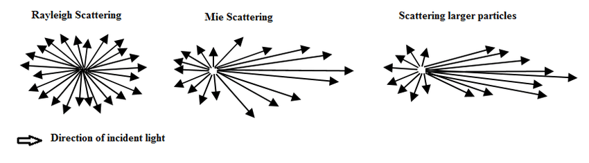
Figure 8 - The angular distribution of the scattered light for the different types of scattering from PhysicsOpenLab.#
In case of spherical particles, with a given refractive index and in case of elastique diffusion, the diffused part of an incident light is expressed using the Mie theory. The intensity and angular distribution is described by a phase function that depends on the scattering regime (Figure 9). For a given wavelenght, big particles diffuse light in the Mie Scattering, wherease smaller particle diffuse light following the Rayleight scattering. Observe your own Mie scattering following the steps given here : PhysicsOpenLab.
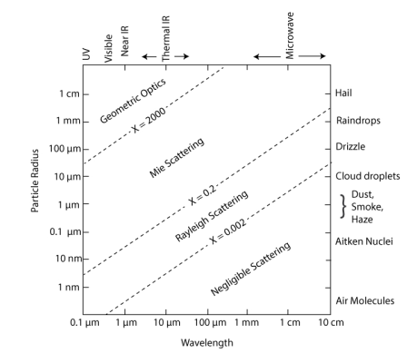
Figure 9 - Scattering regime as a function of the particle size and the wavelength of the incident light, from [Kidder et Haar 1995].#
Therefore, the intensity of the scattered light changes with the angle with respect to the sample.
The three main types of scattering used in turbidity measurements are :
Forward scattering (0-45°): Most sensitive to larger particles
Side scattering (90°): Used in nephelometric measurements
Back scattering (135-180°): Most sensitive to small particles
Note that “larger particles” is defined compared to a wavelength. In tubidity measurement the incident light wavelength depends on the standard! Depending on the wavelength used the scattering measured will be sensitive to slightly different particles size. In coastal areas, forward scattering is typically observed because the particles are usually larger than the wavelength.
Transmissiometry#
▶ Principle
Light attenuation, i.e. the reduction in light intensity, is measured by a light detector positioned at 180° from the light source. This method of turbidity measurement is called transmissiometry. Light attenuation involves both scattering and absorption.Light absorption occurs when particles in water convert incoming light into other forms of energy (typically heat or re-emission at different wavelengths). As light passes through turbid water, suspended particles absorb photons at specific wavelengths, reducing the transmitted light intensity (Figure 7).
The amount of light absorption depends on:
Particle composition (organic vs inorganic matter)
Particle size
Light wavelength
Particle concentration
Different materials absorb light at distinct wavelengths, which is why turbidity sensors often use specific wavelengths to target certain types of particles.
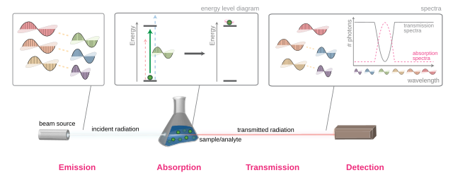
Figure 7 - Overview of light absorption in a sample. White light containing multiple wavelengths passes through the sample. Some wavelengths are absorbed by particles (green light in this example), while others pass through (red light). The transmitted light’s color is complementary to the absorbed wavelengths. From Wikipedia (CC BY-SA 3.0).#
The concentration of the substance is proportionnal to the light attenuation through the modified Beer–Lambert law. See more about optic sensing in [Jacquet 2024].
Optic sensing summary#
In summary, depending on the standard, the method and light emitted in turbidity measurement vary (see Figure 10). Depending on the position of the receptor with respect to the emission either the transmitted or scattered light is measured. The instrument calibration is not based on optical properties but on the degree of turbidity measured in a sample of polymer-based calibration standar. More on turbidity measurement and evolution in [Kitchener et al. 2017]
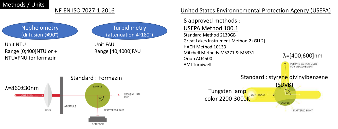
Figure 10 - Summary on turbidity methods and units - by M.Jacquet#
▶ The different type of sensors
Light Sources
Light Emitting Diodes (LEDs)
Most common choice for DIY projects
Advantages:
Low cost and widely available
Long lifetime (>50,000 hours)
Low power consumption
Precise wavelength selection
Common wavelengths:
860 nm (ISO 7027 standard)
850 nm (alternative IR)
White LED (EPA Method 180.1)
Important specifications:
Beam angle (typically 15-30°)
Output power
Wavelength tolerance
Incandescent Lamps
American norm (EPA Method 180.1)
Higher power consumption
Heat generation
Shorter lifetime
Light Detectors
Photodiodes
Types:
PIN photodiodes: Good general purpose
Avalanche photodiodes: Higher sensitivity but more complex
Key specifications:
Spectral response range
Dark current
Response time
Active area size
Phototransistors
Alternative to photodiodes
Higher sensitivity but slower response
More temperature sensitive
Good for high-turbidity applications
Light Dependent Resistors (LDR)
Simplest to implement
Limited accuracy
Slow response time
Temperature sensitive
Good for proof-of-concept projects
▶ Typical characteristics
Key specifications for optical turbidity sensors:
Measurement Range:
Low range: 0-50 NTU (drinking water)
Mid range: 0-1000 NTU (environmental monitoring)
High range: 0-4000 NTU (industrial processes)
Resolution:
Typically 0.01-0.1 NTU for low range
1 NTU for high range
Response Time:
Usually <5 seconds
Faster in continuous flow systems
Light Source:
LED (most common, long life)
Tungsten filament (traditional, broad spectrum)
Infrared (less affected by color)
Sample Volume:
Usually 10-50 mL
Flow-through systems: continuous measurement
▶ Advantages and limitations
Advantages:
Direct measurement of water clarity
Quick response time (<5 seconds)
Wide measurement range (0.01-4000 NTU)
Non-destructive measurement
Well-established standards and calibration methods
Limitations:
Affected by water color and dissolved substances
Bubble interference can cause false readings
Regular calibration required (typically every 3-6 months)
Biofouling in long-term deployments
Temperature sensitivity of light source and detector
Different standards (EPA vs ISO) give different results
Cannot distinguish particle types directly
▶ References
You can access publications and book references via the library’s search tool.
Book
Kidder, S. Q.; Haar, T. H. V. Satellite Meteorology: An Introduction; Elsevier, 1995.
Research article
Kitchener, B. G.; Wainwright, J.; Parsons, A. J. A Review of the Principles of Turbidity Measurement. Progress in Physical Geography: Earth and Environment 2017, 41 (5), 620–642. doi
Thesis
Jacquet, M.; Pellen, F. Développement d’un turbidimètre optique autonome, in situ et à bas-coût, 2024 accessible here.
Website
The Physicsopenlab : https://physicsopenlab.org/2019/07/10/light-scattering/
Other articles to validate :
Contribution needed : Part of this list is taken from ChatGPT 4 and should be double checked :
Comprehensive guide on turbidity measurements Includes detailed specifications for field instruments Discusses measurement ranges and accuracy requirements for different applications These papers would help validate or adjust the specifications currently listed particularly regarding:
Measurement ranges Resolution values Response times Sample volume requirements Light source specifications
Omar, A. F., & MatJafri, M. Z. (2009). “Turbidimeter design and analysis: A review on optical fiber sensors for the measurement of water turbidity.” Sensors, 9(10), 8311-8335. doi
Lambrou, T. P., Anastasiou, C. C., & Panayiotou, C. G. (2009). “A nephelometric turbidity system for monitoring residential drinking water quality.” In Sensor Applications, Experimentation, and Logistics (pp. 43-55). Springer.
Trevathan, J.; Read, W.; Schmidtke, S. Towards the Development of an Affordable and Practical Light Attenuation Turbidity Sensor for Remote Near Real-Time Aquatic Monitoring. Sensors (Basel) 2020, 20 (7), 1993. doi
Metzger, M.; Konrad, A.; Blendinger, F.; Modler, A.; Meixner, A. J.; Bucher, V.; Brecht, M. Low-Cost GRIN-Lens-Based Nephelometric Turbidity Sensing in the Range of 0.1–1000 NTU. Sensors 2018, 18 (4), 1115. doi
Acoustic sensing#
Acoustic methods are used for turbidity measurements, although optical methods remain the preferred approach. Acoustic methods measure total suspended matter rather than turbidity, which correlates more closely with SSC, but requires careful calibration of the materials. Like optical sensing, acoustic sensing is sensitive to sediment characteristics (shape, size, types). Due to this complexity, optical technologies remain the preferred choice for measuring turbidity and SSC [Matos 2024].
▶ Principle
Sound and particle interaction
Acoustic methods for measuring turbidity and suspended sediment concentration (SSC) rely on the interaction between sound waves and suspended particles in water. When acoustic waves encounter particles, they undergo scattering, absorption, and attenuation processes that are dependent on particle characteristics such as size, density, shape, and concentration.
Acoustic backscatter principles
Acoustic backscatter systems emit sound pulses at specific frequencies and measure the intensity of sound reflected back from suspended particles. The signal excess is related to the concentration and properties of particles in the water column. The fundamental relationship is described by the sonar equation:
\(SE = SL - 2TL + Sv - (NL-DI) - DT\)
where:
\(SE\) is the Signal Excess, or signal-to-noise ratio (dB)
\(SL\) is the source level, which relates to the intensity at a distance from the source
\(TL\) is the transmission loss, which depends on an absorption coefficient and distance from the source
\(Sv\) or \(TS\) is the volume backscattering strength or target strength
\(NL\) is the noise level
\(DI\) is the directivity Index
\(DT\) is the detection threshold
The volume backscattering strength (\(S_v\)) is related to particle concentration.
This equation includes acoustic signal corrections for geometry compensation, spherical spreading, and water and particle attenuation. For examples of application with Acoustic Doppler Current Profiler (ADCP), see [Fettweis et al. 2019 or Tessier et al 2008].
▶ The different types of sensors
The sensing element in acoustic backscatter sensors is an acoustic transducer. It can be either a piezoelectric transducer, which converts pressure into electric signal, or an electromagnetic acoustic transducer [Smerdon et al. 1998]. Since acoustic technologies measure a variety of variables (temperature, velocity, bathymetry, etc.), a section dedicated to DIY acoustic instruments and associated sensors is under construction. In this section, we list the acoustic instruments commonly used to measure sediment transport and provide references with useful methodology.
The LISST-ABS is the most common acoustic backscatter sensor used to measure total suspended matter by measuring the amount and size of suspended sediment (which is different from turbidity) ([Mattos 2024] and see a list of research papers using LISST-ABS).
The ADCP is also commonly used to measure SSC due to its colocated velocity measurements over the water column. However, the calibration and data analysis are complex [Tessier C. 2006].
The Acoustic Concentration and Velocity Profiler (ACVP) [Hurther et al. 2011].
The Acoustic Doppler Velocimeter (ADV) is another instrument which measures velocity and turbidity at high rates and single points, making it valuable for turbulence studies [Contribution needed - XXX].
Frequency dependence
The choice of acoustic frequency significantly affects the measurement sensitivity to different particle sizes:
High frequencies (>1 MHz): More sensitive to small particles (clay, silt), shorter range (Figure below)
Low frequencies (75-300 kHz): Better for larger particles (sand), longer range, deeper penetration
Multi-frequency systems: Allow discrimination between particle size classes
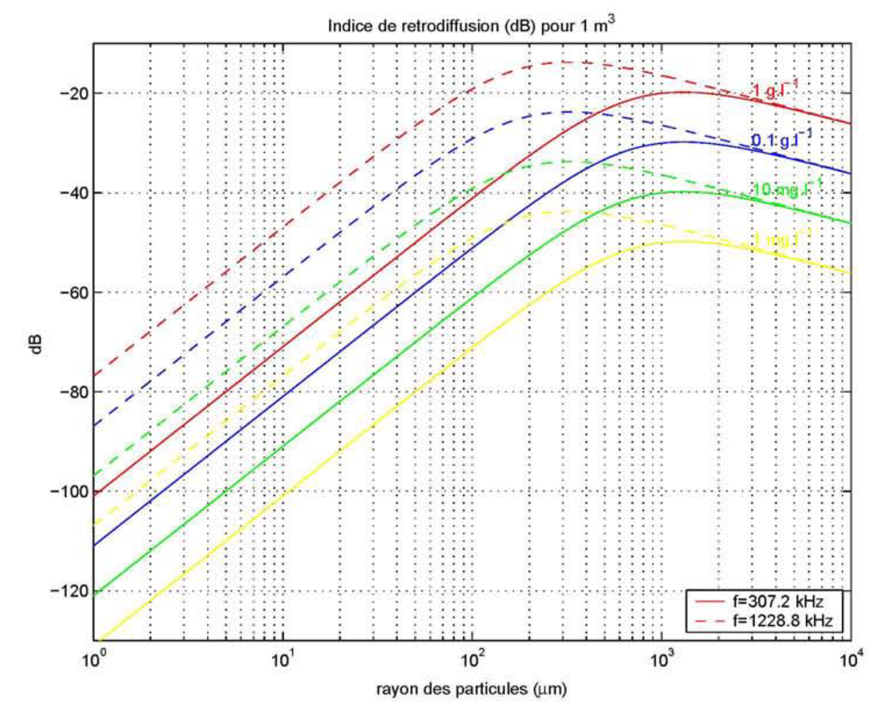
Figure - Volume backscatter index as a function of particle radius for mass concentrations from 1mg/L to 1 g/L, for two different frequencies. Mineral particles. From [Tessier C. 2006]#
▶ Advantages and limitations
Advantages:
Estimates SSC at different depths
Multi-frequency acoustic technologies allow differentiation of sediment particle sizes
Less affected by fouling than optical sensors
Multi-parameter capability: Simultaneous velocity and turbidity measurements
Limitations:
Calibration complexity: Instrument calibration of the emitted and backscatter signals is required for accurate SSC conversion, which can be delicate and time-consuming (Tessier 2006)
Particle size dependency: Response varies significantly with particle size distribution
Stratification effects: Sound speed variations affect measurements
▶ References
Matos, T.; Martins, M. S.; Henriques, R.; Goncalves, L. M. A Review of Methods and Instruments to Monitor Turbidity and Suspended Sediment Concentration. Journal of Water Process Engineering 2024, 64, 105624. doi.
Fettweis, M.; Riethmüller, R.; Verney, R.; Becker, M.; Backers, J.; Baeye, M.; Chapalain, M.; Claeys, S.; Claus, J.; Cox, T.; Deloffre, J.; Depreiter, D.; Druine, F.; Flöser, G.; Grünler, S.; Jourdin, F.; Lafite, R.; Nauw, J.; Nechad, B.; Röttgers, R.; Sottolichio, A.; Van Engeland, T.; Vanhaverbeke, W.; Vereecken, H. Uncertainties Associated with in Situ High-Frequency Long-Term Observations of Suspended Particulate Matter Concentration Using Optical and Acoustic Sensors. Progress in Oceanography 2019, 178, 102162. doi.
Tessier, C.; Le Hir, P.; Lurton, X.; Castaing, P. Estimation de La Matière En Suspension à Partir de l’intensité Rétrodiffusée Des Courantomètres Acoustiques à Effet Doppler (ADCP). Comptes Rendus Geoscience 2008, 340 (1), 57–67. doi.
Tessier, C. Caractérisation et dynamique des turbidités en zone côtière : l’exemple de la région marine Bretagne Sud.
Historical sensing#
The first quantitative methods for measuring water clarity were developed in the 19th century. Two historical instruments were particularly simple and inexpensive to make. They are no longer used nowadays due to their poor accuracy.
▶ Secchi Disk (1865)
The Secchi disk was invented by Pietro Angelo Secchi, an Italian Jesuit priest and astronomer, while he was conducting transparency measurements in the Mediterranean Sea aboard the papal yacht L’Immacolata Concezione. The device consists of a circular disk, painted in contrasting black and white and attached to a measuring line or rope (Figure below).
The measurement procedure is simple:
Lower the disk into water from the shaded side of a boat
Record the depth at which the disk disappears from view
Raise the disk until it reappears and record this depth
Average the two depths to obtain the Secchi depth
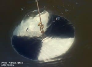
Figure - Picture of a Secchi disk by Adrian Jones - from Magnolia fisheries website#
▶ Jackson Turbidimeter (1900)
Developed by Wilbur Jackson for the water industry, this was the first standardized method for quantitative turbidity measurement. The device consisted of a long glass tube with a flat bottom, a standard candle as light source and a graduated scale (Figure below).
Operating principle:
Pour the sample into the tube
Observe the candle flame from above
Add or remove water until the flame image just disappears
Read the water depth from the graduated scale
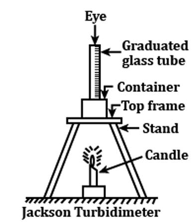
Figure - Schematic of a Jackson turbidimeter#
This led to the Jackson Turbidity Unit (JTU).
Available sensors and instruments#
This table is a list of instruments and sensor to measure turbidity.
• Drag & Drop: Click and drag column headers to reorder columns
• Links: URLs are converted to clickable red cross (✕) icons
| Technology ⇄ | sensor name ⇄ | Type ⇄ | absolute accuracy ⇄ | Range ⇄ | relative accuracy ⇄ | Response time ⇄ | max sampling frequency ⇄ | stability ⇄ | validation level ⇄ | link to validation document ⇄ | mecanical integration ⇄ | maximum depth ⇄ | electronical integration communication interface ⇄ | cost ⇄ | Datasheet link ⇄ | supplying company ⇄ |
|---|---|---|---|---|---|---|---|---|---|---|---|---|---|---|---|---|
| Optical back-scattering | ECO NTU ECO BB | instrument | NC | 250;500;1000 NTU 5 /m | NC | NC | 8 Hz | NC | NC | NC | Diameter : 6.3 cm Length : 12.7 cm (std) ; 17.68 cm (deep) Materials : Acetal copolymer (std) ; Titanium (deep) | 300 m (models B, S and SB) 600m (std) 6000m (deep) | Analog signal : 0-5 V DAQ : 14 bits (16380 counts) Connector : MCBH6MP Communication : RS-232 (19200 baud) | 11 000 € (Feb., 2024) | ECO NTU Turbidity Sensor ECO Scattering Sensor | SeaBird Scientific |
| Optical back-scattering | STM-S | instrument | NC | 25;125;500;4000 FTU | NC | 0.1 s | NC | NC | NC | NC | Diameter : 25.4 mm Length : 66.5 mm (connector version) ; 56.4 mm (bulkhead version) Material : rigid polyurethane, epoxy | 6000 m | Output : 0-5 V Connectors : AG306, MCBH6M, bulkhead | 2 340 $ (Sep., 2024) | Seapoint Turbidity Meter | Seapoint Sensors, inc. |
| Optical side-scattering | ClariVUE10 | instrument | 0.5 FNU | 4000 FNU | ±2% | 9 s | NC | NC | NC | NC | Diameter : 30.1 mm Length : 166 mm Material : Delrin plastic | 30 m | Connector : Bronze 3-pin wet-mate Communication : SDI-12 | NC | ClariVUE10 Product Brochures | Campbell Scientific |
| Optical back-scattering | WiSens TBD | instrument | 0.4 FNU | 4000 FNU | 0,5 % | NC | 1 Hz | NC | NC | NC | Diameter : 45 mm Length : 220 mm | 300m | Communication : WiFi | 5 100 € (Dec., 2019) + wiper : 2 600 € (Dec., 2019) | WiSens TBD Datasheet | NKE Instrumentation |
| Optical back-scattering | Turbidity Plus | instrument | 0 – 10 NTU (+/- 0.1 NTU) 10 – 1000 NTU (+/- 0.4 NTU) | 3000 NTU | > 1000 NTU (+/- 0.04% of NTU) | < 3 s | NC | NC | NC | NC | Diameter : 3.01 cm Length : 15.49 cm Material : Delrin | 200 m | Signal output : 0-5 V | 1 327 € (Apr., 2019) | Turbidity Plus Product Datasheet | Turner Designs |
| Optical transmissiometry | SEN0189 | sensor | NC | NC | NC | < 500 ms | NC | NC | NC | NC | Diameter : 27.8 mm Length : 34.1 mm Material : PP | NO waterproof | Analog output : 0-4.5 V Digital output Connector : molex | nearly 10 € | SEN0189 Datasheet | DF ROBOT |