Temperature#
The “Background” section summarises typical characteristics of temperature encountered in the ocean : the temperature range, vertical profile, and spatial and temporal scales encountered in the ocean. Temperature measurements can be taken by “Contact sensing” (using sensors such as thermistors, thermocouple and RTDs (resistance temperature detectors)) or with “Remote sensing” by measuring thermal radiation (e.g. satellite measurements or thermal cameras).
The “Historical and high-technology sensors” section presents technologies no longer used today or that are not suitable to DIY approache. Finally, a table of sensors and instruments available on the market is provided in the “Sensors databse” section.
Contributions:
Background#
Ocean temperature ranges between -2°C and 40°C globally. It controls the evolution of ocean circulation, climate systems, and marine habitats. Temperature determines water density (together with salinity and pressure) and hence conditions the oceanic circulation [section 1.2.4 Siedler 2001]. It reflects the amount of energy stored and absorbed by oceans [Cheng et al. 2020].

You can measure temperature for a variety of purposes and key climate indicators directly linked to temperature measurements include sea surface temperature (SST), ocean heat content, and indicators of marine heat waves. Discover typical variations of temperature depending on location, height above sea floor and time and the evolution of temperature standard! Use this section to warm-up before learning about temperature sensors technology!
▶ SST
Temperature varies in general with depth, location, and time. Sea surface temperature ranges between 2°C and 32°C (Figure 1). SST is routinely observed using satellite measurements. Modern satellites can achieve horizontal resolution down to about 100 m. However, not all satellites reach this resolution. Measurements are more difficult near coasts and under clouds. In situ measurements fill in the gaps.
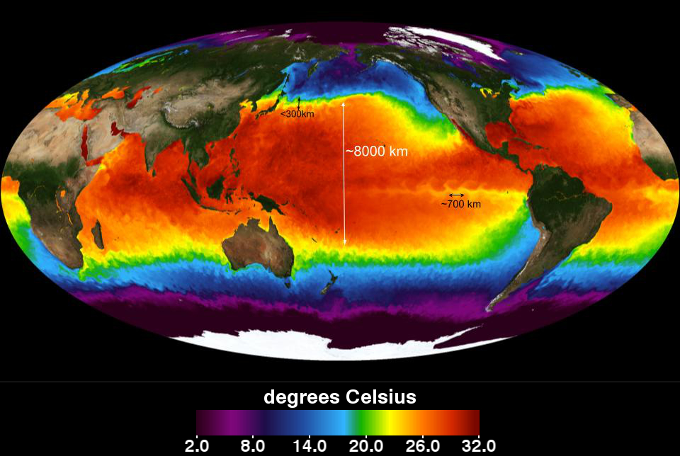
Figure 1 - Observations of Multiscale Ultra Resolution Sea Surface Temperature. Data combines satellite measurements with surface observations from ships and buoys - source: NASA/Goddard Space Flight Center#
▶ Vertical profile
Variation of heat input and mixing processes of various temporal scales affect the vertical temperature profile. The strongest vertical temperature gradient occurs in the first tens of meters below the surface (Figure 2). This region is called the thermocline. Thermocline strength increases seasonally with sun and atmospheric heat input variations. A temperature change of 10°C between 0 m and about 100 m depth is easily observed in summer. At the coast, in water depths less than 200 m, a secondary weaker thermocline sometimes forms near the bottom due to bottom friction. At greater depths, temperature slowly decreases. Variations of 10°C occur over more than 1 km depth (Figure 2, [CH. 7 Bowden 1983]).
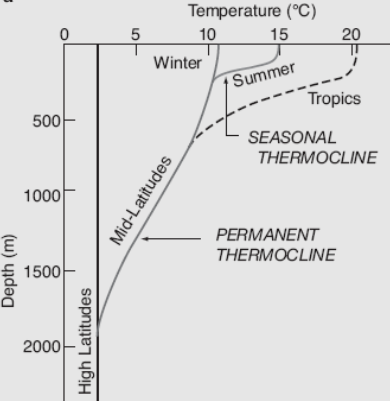
Figure 2 - Different thermocline profiles (temperature versus depth) based on season and latitude - from the Wikipedia page of Thermocline#
▶ Time series
The scale of temperature variations is not the same at each temporal scale. Seasonal variations are on the order of 1°C, monthly trends are on the order of 0.5°C, and daily changes are around 0.1°C, which matches the sensor precision (Figure 3).
The data presented in Figure 3 are taken from the COAST-HF-MAREL-Iroise buoy, which monitors the coastal ecosystem of the Bay of Brest at high frequency (subhourly) and for the long term (since 2000). Temperature measurements are made with an MP7-NKE probe that uses a WTW (thermistor) sensor for temperature, which provides 0.1°C precision.
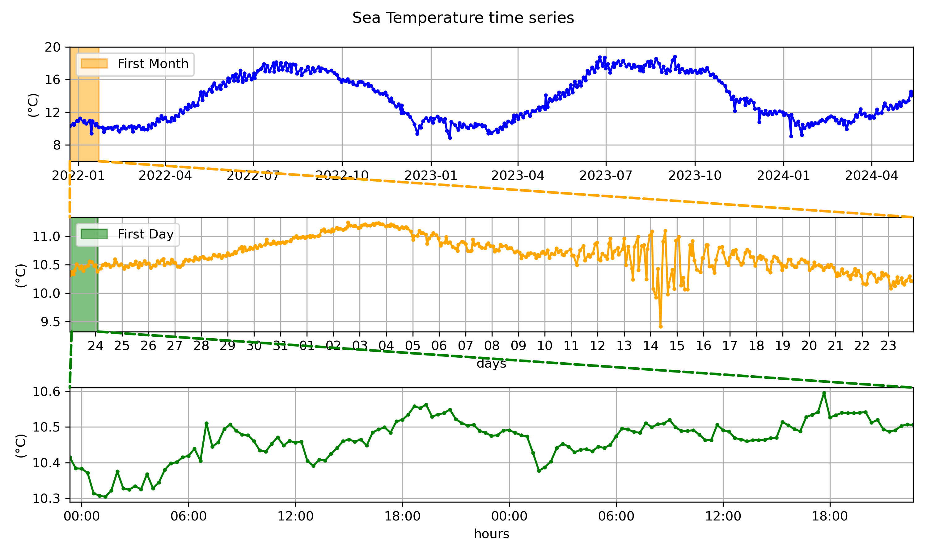
Figure 3 - COAST-HF-MAREL Iroise buoy sea temperature measurement at [48.35796°, -4.55175°] doi - by [Rimmelin-Maury et al.(2023)]. The complete data set can be viewed on the Coriolis website#
▶ Temperature Standards
Temperature System International (SI) Unit is the kelvin (K). The kelvin (K) is defined by taking the fixed numerical value of the Boltzmann constant \(k\) to be \(1.380 649 x 10^{−23}\) when expressed in the unit J K−1. The most recent International Temperature Scales (ITS) internationally adopted is the ITS-90 [BIPM (2019) ; Preston-Thomas (1990)]. One of the standard for temperature calibration is the triple point of water (273.16 K) [Preston-Thomas (1990)].
International temperature scales have evolved over the years. This is particularly important when comparing historical measurements. Temperatures using the International Practical Temperature Scale 1968 (IPTS-68) differ from those using the Internaltional Temperature Scale of 1990 (ITS-90) by up to 0.01°C within oceanographic ranges. Further information on temperature definitions, measurement standards and the evolution of the seawater equation of state can be found in Pawlowicz (2013). Comparisons between actual and historical data should be made with particular attention to the standards used.
▶ References
You can access publications and book references via the library’s search tool.
Publications
Cheng, L., Abraham, J., Zhu, J. et al. (2020).Record-Setting Ocean Warmth Continued in 2019. Adv. Atmos. Sci. 37, 137–142 . doi
Pawlowicz, R. (2013) Key Physical Variables in the Ocean: Temperature, Salinity, and Density. Nature Education Knowledge 4(4):13. website
Preston-Thomas, H. The International Temperature Scale of 1990 (ITS-90). Metrologia 1990, 27 (1), 3. doi.
Rimmelin-Maury P., Charria G., Repecaud M., Quemener L., Beaumont L., Guillot A., Gautier L., Prigent S., Le Becque T., Bihannic I., Bonnat A., Le Roux J-F., Grossteffan E., Devesa J., Bozec Y., Gautier de Charnacé C. (2023). COAST-HF-Marel-Iroise buoy¿s time series (French Research Infrastructure ILICO) : long-term high-frequency monitoring of the Bay of Brest and Iroise sea hydrology. SEANOE. doi
Books
BIPM. Le Système International d’unités (SI) / - The International System of Units - (SI); 2019. ISBN - 978-92-822-2272-0
Bowden, K.F. (1983) Physical Oceanography of Coastal Waters. Camelot Press Ltd., Southampton, Great Britain, 302 p.
Siedler, G.; Church, J.; Gould, J., eds. (2001), Ocean Circulation and Climate: Observing and Modelling the Global Ocean. San Fransisco CA, USA, Academic Press, 736pp. (International Geophysics Series, 77).
Websites
Multi-scale ultra high resolution sea surface temperature (MUR): URL
Wikipédia
Now you know what to expect in terms of temperature measurement wherever you are! (Or close enough). You should understand that temperature fluctuate at various time and spatial scales. So make sure you clearly define what you want to look at! At this point you can decide what you want to learn from temperature measurements. The next two sections provide simplified theoretical insights into the different sensing elements to help you master the technology and understand its advantages and limitations.
Contact sensing#
Contact thermal measurements mainly use an electric component which react to temperature changes. These sensors are inexpensive and compact. There are three main types:
Thermistors are semiconductors whose resistance changes with temperature. They are commonly used in oceanography due to their good sensitivity. However, the resistance variation with respect to temperature is not linear. See section Thermistor.
Thermocouples produce an electrical current by Seebeck effect which depends on the temperature environment. Thermocouples are less used then thermistors because of the complex electrical circuit involved. However, they are robust and have a fast time response (around 10 ms). See section Thermocouple.
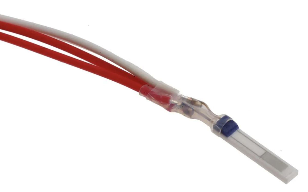
RTDs are metallic wires whose resistance changes with temperature (like the PT100). The resistance variations are small, so they require a more sensitive acquisition system tend than the thermistor. See section RTD.
Thermistor#
The word “thermistor” derives from the description “thermally sensitive resistor”. It was first discovered by M. Faraday in 1833. At this time, mass production of thermistors was challenging, so commercial production only started in the 1930s. The development of high-performance semiconductors in the late 20th century significantly increased sensor sensitivity and precision, as well as expanded the operational temperature range. Today, thermistors are used for a wide range of applications. They are the main type of temperature sensor for oceanographic measurements due to their good precision and low cost.
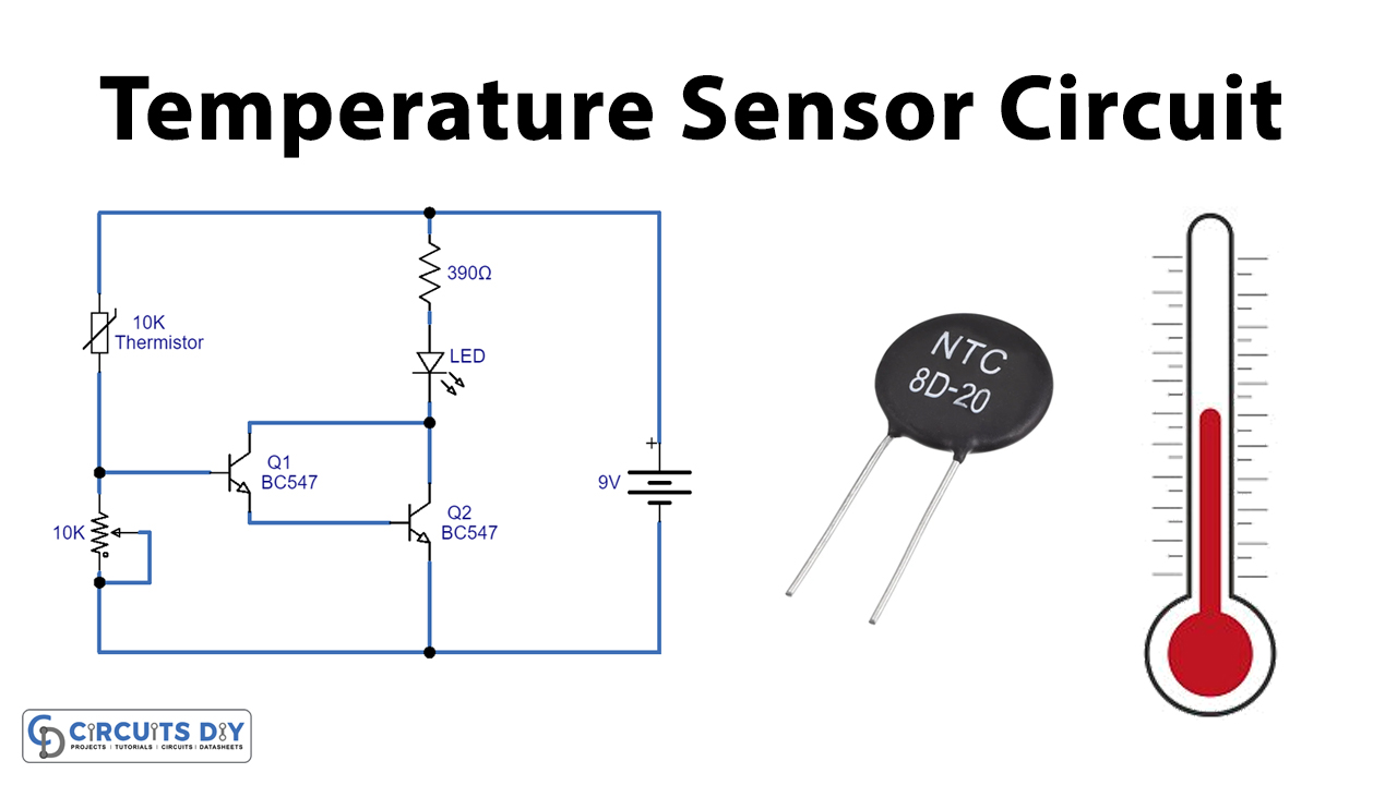
from circuit DIY - temperature sensor circuit using thermistor#
▶ Principle
A thermistor is made of metal oxides pressed into a bead and encapsulated in an impermeable material. This sensor is a semiconductor whose resistance changes nonlinearly with temperature (Figure thermistor curve). The high resistance value makes the thermistors not particularly susceptible to self-heating (compared to the small signals produced by other types of sensors). The change in resistance is relatively large with a temperature changes (-3% to -6% per °C), threfore easy to measure.
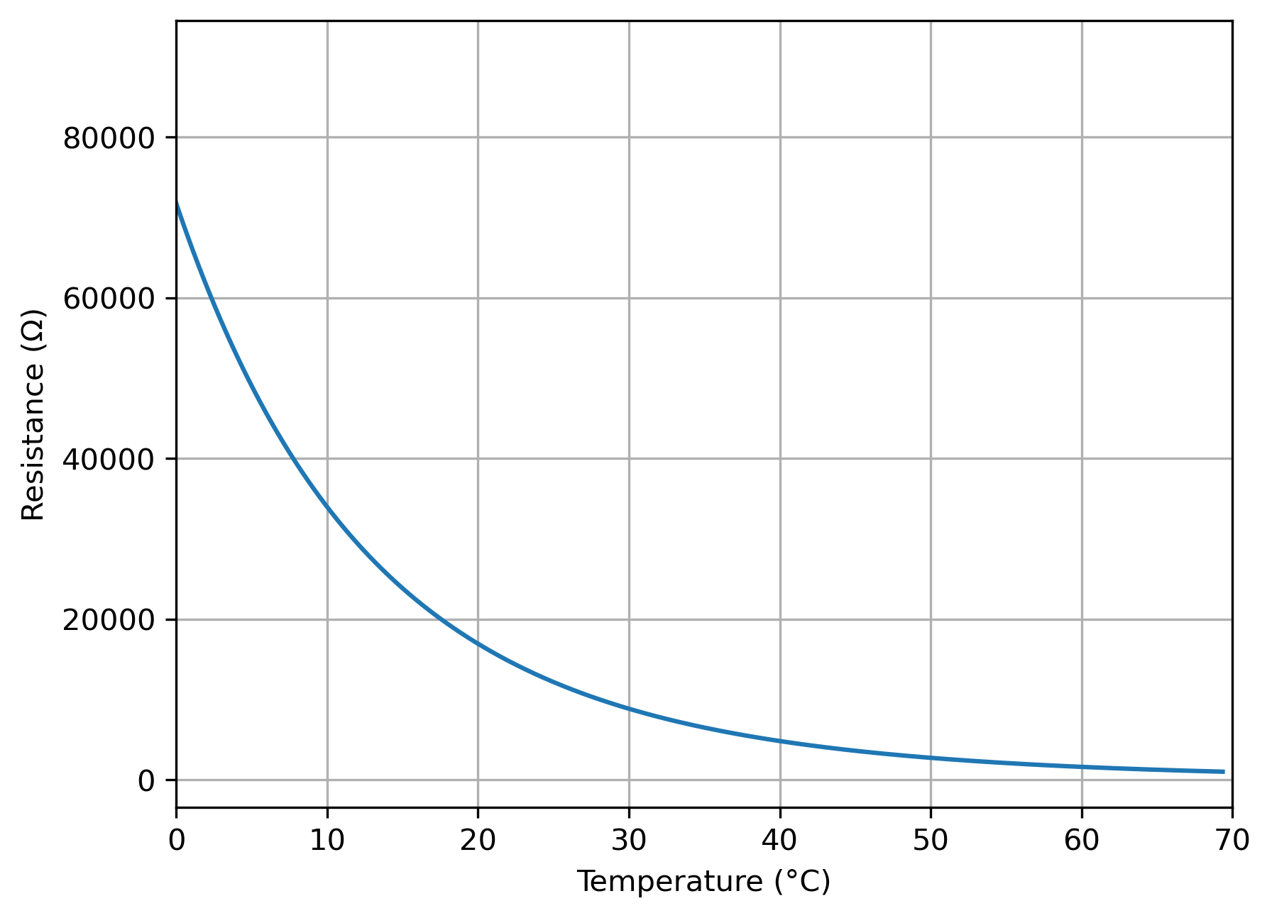
Resistance vs temperature plot for the Steinhart coefficients given for standard part no.1 from BetaTHERM Sensors#
The thermistor is mounted on a circuit, protected, and placed in the environment of interest. The resistance changes as a function of temperature in a nonlinear way described by the Steinhart-Hart equation (named after two oceanographers [Steinhart & Hart (1968)] - more information on the general approximations used in the Steinhart-Hart equation can be found in NTC Thermistor theory by BetaTHERM):
Where \(T\) is in Kelvin and \(A\), \(B\) and \(C\) are constants that depend on the individual thermistors.
Constant temperature baths are used to calibrate the thermistor. In each bath (at least 3, preferably 5), the temperature is measured with another device and linked to the thermistor resistance. The measurements are used to compute the values of \(A\), \(B\) and \(C\). Note that the Steinhart-Hart equation is used by all thermistor manufacturers (see BetaTHERM or DXM website). The offset is generally constant and depends on the sensor, and needs to be measured beforehand.
▶ The different types of sensors
Negative temperature coefficient (NTC or CTN) thermistors decrease in resistance as temperature increases. NTC thermistors are the most commonly used sensors. (see more about NTC thermistor in EE Power). Positive temperature coefficient (PTC or CTP) thermistors increase resistance as temperature increases.
NTC thermistors are made by combining powdered metal oxides (manganese, nickel, cobalt, copper) with stabilizing agents in an organic binder solution. The composition of the metal oxides and stabilizers determines the final thermistor’s resistance-temperature characteristics and electrical properties. The mixture is then baked, cut and coated with an electrode material. Lead wires with low thermal conductivity can then be added if needed. A detailed description of the manufacturing process can be found on the Littelfuse website. The final coating (usually epoxy resin) protects the thermistor from external corrosion. Each step affects the final thermistor characteristics.
Glass-isolated thermistors enable temperature microstructure measurements with resolution below \(10^{-5}K\) but they are highly sensitive to mechanical stress [sect 12.5 in Baumert 2005].
▶ Typical characteristics
Time response: 7 ms - 3 s - 15 s. Depends on the flow speed, the thermistor size and materials. See more about dynamic response of glass rod thermistor in [Gregg et al. 1980].
Sensitivity: down to \(10^{-5}K\) [Baumert 2005]. Otherwise [-3% to -6%] changes in reistance per °C. It depends on the isolation method (see BetaTHERM for more information)
Size: 0.075 - 5 mm
▶ Advantages and limitations
Advantages:
Resistance value is easy to measure: no need for amplification
Good sensitivity
Inexpensive
Widely used and developed in oceanography
Limitations:
Nonlinear resistance versus temperature
Requires careful calibration
Poor interchangeability compared to RTD [Lin et al. 2004] and because offset is sensor dependent [communication with P.Lazure]
Sensors may be sensitive to mechanical stress
▶ References
You can access publications and book references via the library’s search tool.
Papers
Gregg, M. C., and T. B. Meagher (1980), The dynamic response of glass rod thermistors, J. Geophys. Res., 85(C5), 2779–2786, doi
John S. Steinhart, Stanley R. Hart, 1968: Calibration curves for thermistors, Deep Sea Research and Oceanographic Abstracts, Volume 15, Issue 4, Pages 497-503, ISSN 0011-7471, doi
Lin, X., and K. G. Hubbard, 2004: Sensor and Electronic Biases/Errors in Air Temperature Measurements in Common Weather Station Networks. J. Atmos. Oceanic Technol., 21, 1025–1032, doi
Lazure P., Le Berre D., Gautier L. 2015: Mastodon Mooring System To Measure Seabed Temperature Data Logger With Ballast, Release Device at European Continental Shelf . Sea Technology , 56(10), 19-21 . Open Access version
Wolk, F., H. Yamazaki, L. Seuront, and R. G. Lueck, 2002: A New Free-Fall Profiler for Measuring Biophysical Microstructure. J. Atmos. Oceanic Technol., 19, 780–793, doi
Conference papers
Khan, Md & Burnett, Matthew & Downey, Austin & Satme, Joud & Imran, Jasim. (2025). UAV deployable buoy-style sensor for in situ water quality monitoring. 14. doi & PDF
Books
Marine Turbulence—Theories, Models, and Observations, Results of the CARTUM Project, edited by H.Z. Baumert, J.H. Simpson, and J. Sündermann, Cambridge University Press, 2005, 672 pages, ISBN 0521837898
Websites
Thermocouple#
Thermocouples produce an electrical signal due to temperature changes that can be transmitted and processed electronically. Thermocouples are inexpensive and easy to construct (see video How to make a Thermocouple or the blog Making a thermocouple).
Thermocouples are robust sensors that can operate over a wide temperature range and be smaller than a few micrometres. However, any change in lattice structuree or impurity modifies the amount of generated voltage making the sensor less accurate [Pavlasek et al. 2015].
They are typically employed in industrial processes as well as in healthcare applications [Zhang et al. 2022 ; Leonidas et al. 2022]. In the metallurgy industry, thermocouples are slower and less precise than the infrared thermometers and fibre obtics [Leonidas et al. 2022] and drift (0.22°C per hour above 100°C - [Pavlasek et al. 2015]).
In oceanography, thermocouples offer an interesting spatial resolution and a fast response times (in the order of the milliseconds) compared to thermistors and to RTDs. They are well suited to use as microstructure sensors at sites with pronounced thermal stratification [Nash et al. 1999]. Currently, no studies using thermocouples for long-term measurements have been found. Despite the need for complex electronic development, thermocouples are suggested as an interesting sensor to develop in oceanography. Contributions are welcome.
▶ Principle
Thermocouples work based on the Seebeck effect, where a voltage is generated at the junction of two dissimilar metals when there is a temperature difference between the junction and the ends of the metals. Electrons spontaneously migrate towards the colder area and, because the two metals have distinct electrical properties the voltage is different between the two ends of each metal. The potential difference between the two metals is called the contact electromotive force (EMF). The EMF produced depends on the metals and is proportional to the temperature difference. No voltage is measured if the two metals are similar or if there is no temperature difference. Standard couples of metals are usually used (see tcaus website for more information on thermocouple standards). A detailed description of thermocouple construction can be found in [Marmorino et al. 1977].
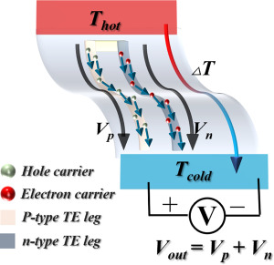
Principle of temperature measurement in flexible thin-film thermocouples by [Zhang et al. 2022]. Note that \(T_{cold}\) is known.#
Thermocouples are placed at the desired location to measure temperature. The cold end provides the reference temperature \(T_{ref}\) and must be measured (using another temperature sensor), whereas the voltage is measured at the hot end. The reference temperature is then used to compensate the voltage measured at the “hot” end. Finally, the thermocouple is either calibrated or its calibration curve is used to obtain the “hot” temperature knowing the voltage output. The voltage measured is a few mV (Figure Thermocouple voltage) and is usually amplified, which adds noise.
In two examples, thermocouples were counstructed in-house and mounted on profilers falling at 1 m/s and measured vertical temperature gradients [Nash et al. 1999], [Marmorino & Caldwell 1978]. In Nash et al. (1999) the final sampling rate was 102.4 Hz. Thermocouples showed less variance than thermistors in turbulent patches within large temperature-gradient signal. In both studies, the noise due to signal amplification limited the measurement accuracy. Future improvements in operational amplifiers could enhance performance (see Figure 12 in [Nash et al. 1999]).
▶ The different types of sensors
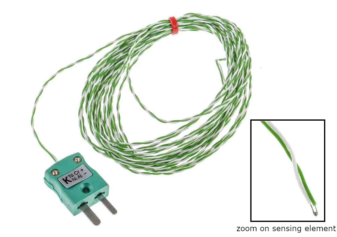
Thermocouples are available in various types (e.g., Type K, Type T, Type J) depending on the metals used and the temperature range.
In oceanography, chromel-constantan thermocouples (ANSI type E) are preferred since they have the highest EMF of any standard metallic thermocouple at typical oceanic temperatures [Marmorino & Caldwell 1978].
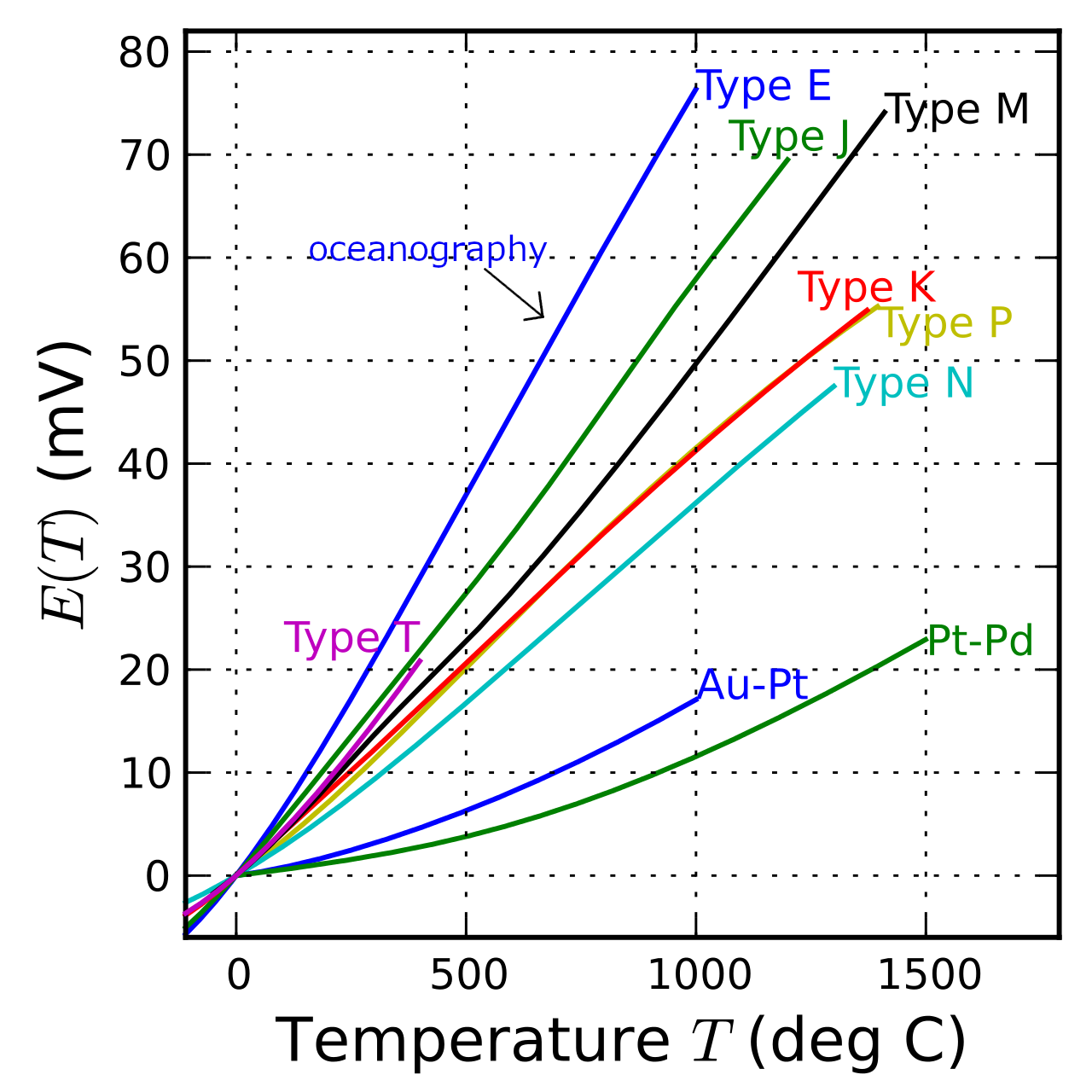
Thermocouple voltage (E(T)) as a function of temperature - from Instrumentation hub website#
▶ Typical characteristics
Accuracy: 0.75 mK in situ [Nash et al. 1999], after amplification. It depends on the amplifiers.
Time response: less than 0.8 ms in [Nash et al. 1999] and around 0.06 s in [Marmorino & Caldwell 1978] (note that they take into account the effect of the fluid boundary layer).
Sensitivity: around 60 \(\mu V / K\) at \(10°C\)
Size: μm
▶ Advantages and limitations
Advantages:
Robust
Fast time response
No need to be electrically insulated from the fluid
Limitations:
Low sensitivity : can be increased by arranging thermocouples in series [Baumert 2005]
Multiple sources of errors: thermal contact between the cold junction compensator and the reference junctions can lead to errors in the computed temperature and errors in \(T_{ref}\) measurements.
Profiler measurements: no tests on moorings maybe due to drift. Maximum 30h of field use in [Marmorino & Caldwell 1978].
▶ References
You can access publications and book references via the library’s search tool.
Publications
E. Leonidas, Ayvar-Soberanis S, Laalej H, Fitzpatrick S, Willmott JR. (2022). A Comparative Review of Thermocouple and Infrared Radiation Temperature Measurement Methods during the Machining of Metals. Sensors (Basel). doi
G. O. Marmorino, D. R. Caldwell, 1978. Horizontal variation of vertical temperature gradients measured by thermocouple arrays, Deep Sea Research, Volume 25, Issue 2, Pages 221-230, ISSN 0146-6291, doi
J. D. Nash, D. R. Caldwell, M. J. Zelman, and J. N. Moum, 1999: A Thermocouple Probe for High-Speed Temperature Measurement in the Ocean. J. Atmos. Oceanic Technol., 16, 1474–1482, doi
Z. Zhang, Z. Liu, J. Lei, L. Chen, L. Li, N. Zhao, X. Fang, Y. Ruan, B. Tian, L. Zhao, 2023. Flexible thin film thermocouples: From structure, material, fabrication to application, iScience, Volume 26, Issue 8, ISSN 2589-0042, doi
Book
Marine Turbulence—Theories, Models, and Observations, Results of the CARTUM Project, edited by H.Z. Baumert, J.H. Simpson, and J. Sündermann, Cambridge University Press, 2005, 672 pages, ISBN 0521837898
Conference paper
Pavlasek P., Ďuriš S., Palencar R. Selected Factors Affecting the Precision of Thermocouples; Proceedings of the XXI IMEKO World Congress “Measurement in Research and Industry”; Prague, Czech Republic. 30 August–4 September 2015; p. 4. PDF
Website
How to make a thermocouple - https://www.youtube.com/watch?v=-8cBCjJJcB4
Making a thermocouple - https://www.instructables.com/Making-A-Thermocouple/
A brief history of thermoelectrics - https://thermoelectrics.matsci.northwestern.edu/thermoelectrics/history.html
Wikipedia
Thermocouples types and standards: https://www.tcaus.com.au/thermocouple/thermocouple-standards.html
RTD#
RTD stands for Resistance Temperature Detector. It differs from a thermistor in terms its composition and behaviour. RTDs are made of pure metal, the resistance of which changes linearly with temperature. This contact sensor offers relatively good accuracy (around 0.2°C) over time and over a large range of temperatures (usually used between -50°C and 50°C) but it does generate self-heating. RTDs are most commonly used in atmospheric sciences [Lin & Hubbard 2004].
▶ Principle
It is an electrical circuit in which the resistance changes linearly with temperature (Figure courbe R-T).
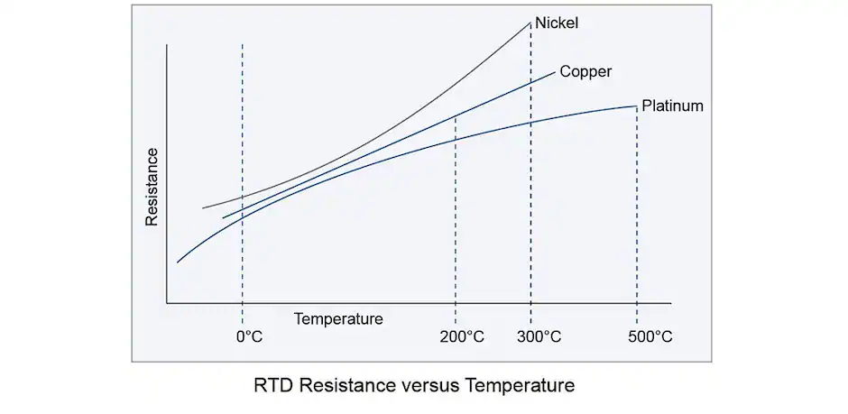
Resistance as a function of the outside temperature for resistive element in a circuit made of Platinum, Copper and Nickel - from TE connectivity website#
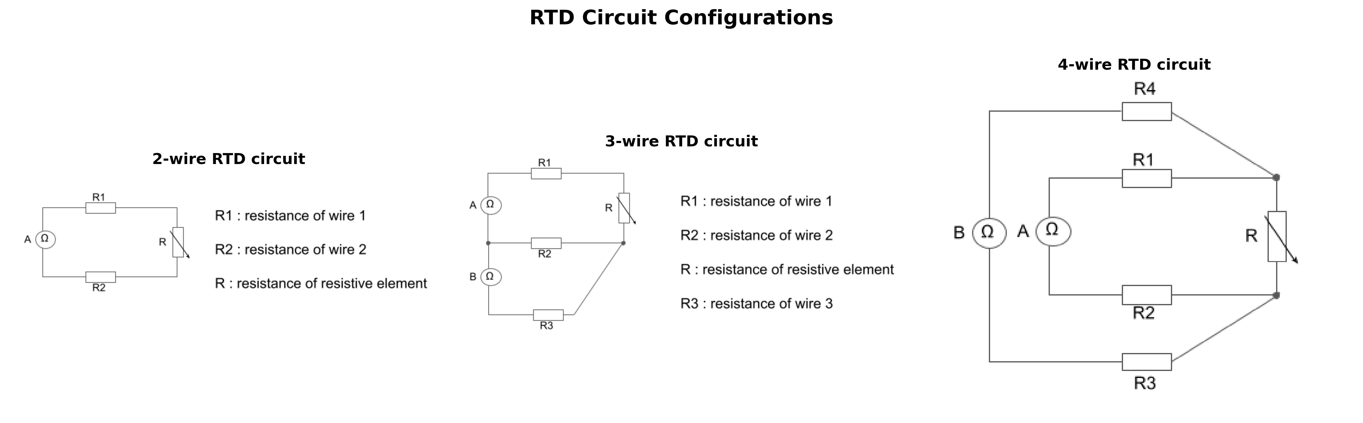
The most basic RTD circuit is a 2-wires circuit, made of a resistive element connected to a power source with two insulated wires and an ohmmeter (Figure ). In a 2-wire circuit, the wire resistances add error to the measurement.
To improve accuracy, RTD circuits with three or four wires are used to compensate for the lead wire resistance. The usual RTD circuit uses 3 wires. Resistance is measured at 2 points by ohmmeter \(A\) and ohmmeter \(B\). Ohmmeter \(A\) measures \(R_1+R+R_2\). Ohmmeter \(B\) measures \(R_2+R_3\). If the three wires are identical with the same temperature, \(R_1=R_2=R_3\), \(A-B=R\). The accuracy of this circuit is around 0.5°C.
Finally, a 4-wires RTD circuit has an accuracy of around 0.15°C.
Depending on the current, the sensor may not be able to dissipate the heat. In this case, the final measurement may be artificially increased. Self-heating error leads to an artificial increase of 0.5°C under 1 m/s airflow in atmospheric measurements [Lin & Hubbard 2004]. The authors suggest improvements such as chill mirror mechanisms to reduce self-heating.
▶ The different types of sensors
Different types of metals are used (Pt, Ni, Cu) in RTDs. Usually, the element used is platinum, which has a 100 \(\Omega\) resistance at 0°C. A change of 1°C corresponds to 0.384 ohm for a Pt100 (see TE website for information on other metals). Platinum is preferred due to its stability. Pt100 can be used for a long period of time without any change in its behavior.
Voltage outputs are small (around 1V). For a Pt100, an error of 100 \(\mu V\) is an error of 0.4°C (see guilcor sensors website for more information on RTD errors and accuracy).
▶ Typical characteristics
This is for a Pt100:
Accuracy: [0.15-0.5°C] depending on the circuit
Time response: 1-1.5s (Endress+Hauser website)
Sensitivity: \(0.1 \Omega / °C\) (see tc website)
Size: 2 mm (RS website)
Calibration: Each year for a specific temperature range in atmospheric measurements [Lin & Hubbard 2004]
▶ Advantages and limitations
Advantages:
Wide range of temperature measurements (-200 - 700°C)
Linear relationship between temperature and resistance
Limitations:
Self heating
The sensor accuracy depends on the electric circuit configuration
Needs regular calibration to check changes in the wire resistance
▶ References
You can access publications and book references via the library’s search tool.
Publications
Lin, X., and K. G. Hubbard, 2004: Sensor and Electronic Biases/Errors in Air Temperature Measurements in Common Weather Station Networks. J. Atmos. Oceanic Technol., 21, 1025–1032, doi
Websites
DIY RTD for a DMM: EDN website.
DIY Resistive Thermal Device - “RTD”: youtube video by Nick Moore.
What is a RTD sensor? - Dracal technologies website
RTD PT199 by RS - RS website
RTD PT100 by Guilcor sensors - Guilcor sensors website
Remote sensing#
Remote sensing measures sea surface temperature (SST) without physical contact. All thermal instruments use the principle of thermal radiation. Different sensor types are based on this principle:
Radiometers
Thermal cameras
Infrared thermometers
Usually, thermal cameras and pyrometers output a temperature with low accuracy (the best I found so far is ±2°C for a thermal camera around 500€). However, combined measurements and dedicated post-processing may significantly increase accuracy [Robinson & Donjon 2010], Zhang & Wang 2022. Remote sensing allows the measurement of skin temperature (0–500 μm below the surface; The thermal stucture within the first few micrometres below the sea surface is complex and different methods of measuring the SST may record different values. Furthermore, object smaller than the IR wavelength may not be approximated by the black body approximation Cuevas 2019). Therefore the following text may not apply to the SST_skin measurement and contributions on SST_skin are more than welcome.
Radiometers measure radiance over several thin spectral bands and provide radiation output. Radiometers are expensive and relatively massive instruments used on satellites or on Earth to measure sea and atmospheric properties. More information about radiometers can be found on the Apogee instrument website and in the Flir website. Radiometers are not considered in the following sections; contributions are more than welcome.
This section first presents the “General principle” of thermal radiation and the “measurement process”. Then we describe the two main affordable instruments: “Thermal camera” and “Infrared thermometer”.
▶ General principle of thermal radiation
Remote temperature measurement aims to capture the intensity of long wavelength emissions from an observed body. Matter naturally emits electromagnetic radiation at different wavelengths which constitutes a spectrum (see Figure solar spectrum). The shape of the spectrum depends on the temperature of the body. The peak emission for instance shifts towards shorter wavelengths as temperature increases as described by Wien’s displacement law (see Figure solar spectrum). The sun, at a temperature of 5900 K, has a maximum luminous intensity in the “visible” wavelengths (from a human point of view), whereas SST whose temperature is between 2 and 32°C does not spontaneously emit in the visible range; but in the infrared and microwave wavelength range. A fun interactive simulation of the blackbody spectrum can be find in the Phet website from university of Colorado. Note that, as you decrease the temperature, you will have to reduce the \(y\) axis limit (i.e reduce the power density) and the \(x\) axis limit (i.e reduce the wavelength towards the IR) in order to accurately observe the shape of the spectrum.
The radiation captured by the instrument is a combination of what is emitted by the body of interest and the environment. When looking at the SST, measurements also capture what the atmosphere emits (and all the other bodies that may be present on the way). The atmosphere emits where it absorbs sunlight (see Figure solar spectrum). Usually, filters are chosen between 10.5–12.5 μm (atmospheric window) to avoid atmospheric absorption bands without being too broad. Once the radiation is corrected, one can compute the temperature associated with the emission using Stefan-Boltzmann’s Law. The approximations made at this stage are : 1) the SST mostly emits in the measured range 2)the spectrum is approximated by the black-body spectrum, described by Planck’s Law.
To better represent the spectrum of a real body, measurements can be taken across several bands (such as in satellite measurements). To better fit the black body spectrum to the real body spectrum more accurately, a correction factor called the emissivity is used. For instance, emissivity of the sea surface will depend on the angle of observation and the surface wind speed Masuda et al. 1988. More information can also be found in [DeWitt & Nutter 1988]. A complete course about atmospheric radiation written by J. Lefrere can be found here. For english readers [Bohren 2005] describe fundamentals of atmospheric radiation with plenty of exercices.
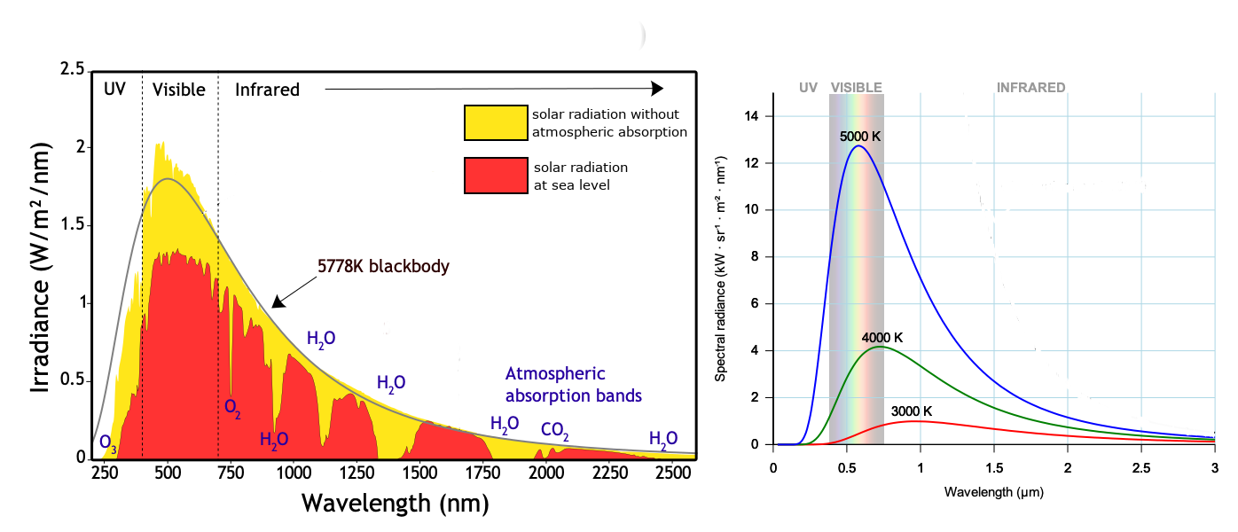
(left) Solar spectrum above the atmosphere (yellow) and at the surface (red), Black body spectrum at the sun’s temperature (black curve) - Adapted from Solar spectrum by Robert A. Rohde. (right) Black body spectral radiance curve for various temperatures adapted from Black body illustration by Darth Kule - Own work, Public Domain#
Compared to contact sensing, thermal radiation is a non-intrusive measurement, which makes it ideal for SST measurement.
▶ Measurement process
The sensor is oriented at a fixed angle towards the object. The lens and filter focus the thermal energy onto the detector. The lens is made of materials highly transparent to IR radiation (such as Germanium or Chalcogenide). If relevant, the lens should be carefully chosen and its effect may be considered. The detector converts the thermal energy into an electric signal. Different types of detectors are used (microbolometers, thermopiles or quantum detectors). A microbolometer is commonly used, it has the slowest response (~10ms) and is the cheapest option. More information can be found in “The Ultimate Infrared Handbook for R&D Professionals”. The electric signal is amplified and can either corresponds to straight radiation (the output : this is radiometric measurements) or temperature after raw signal processing (temperature : thermographic measurements). This is in general an option in radiometers and thermal camera and IR thermometers
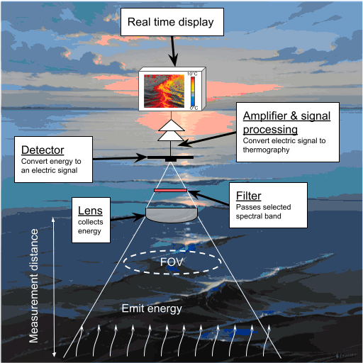
Basic components of a thermal imaging system - adapted from Jo et al. (2013)#
Radiometric measurements allow for accurate SST measurement when carefully post-processed. The main sources of error are : inaccuracy in the representation of the sea surface spectrum (the sea surface is not a black body and its emissivity needs to be characterized) and in the quantification of atmospheric radiation. The lens contribution may also affect the final result (see thermal camera section).
▶ References
You can access publications and book references via the library’s search tool.
Publications
Cuevas, J. Thermal radiation from subwavelength objects and the violation of Planck’s law. Nat Commun 10, 3342 (2019). doi
K Masuda, T Takashima, Y Takayama, 1988. Emissivity of pure and sea waters for the model sea surface in the infrared window regions, Remote Sensing of Environment, Volume 24, Issue 2, doi
D. P. DeWitt, G. D. Nutter, 1988. Theory and Practice of Radiation Thermometry, Online ISBN:9780470172575, doi
Robinson, I. S., & Donlon, C. J. (2003). Global Measurement of Sea Surface Temperature from Space: Some New Perspectives. Journal of Atmospheric & Ocean Science, 9(1–2), 19–37. doi
Zhang, K., & Wang, X. (2022). High-Precision Measurement of Sea Surface Temperature with Integrated Infrared Thermometer. Sensors, 22(5), 1872. doi
Book
J. Lefrere : Rayonnement atmopshérique, télédétection. Cour de Master de Sciences et technologies, Sorbonne université PDF . It contains a complete and accessible bibliography
Bohren, Craig F. et Eugene E. Clothiaux, Fundamentals of Atmospheric Radiation, 472 p. (Wiley-VCH, 2006), ISBN 978-3-527-40503-9. PDF
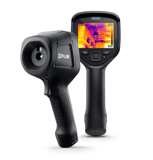
Thermal camera#
Thermal cameras cost around 160–1500€ and can be lightweight (153g), wireless, or plugged into smartphones. Cameras can be technically challenging, and training may be needed to fully handle them. Thermal sensor array can also be purchased see Melexis sensing element which drastically reduce the cost.
▶ Typical characteristics
Accuracy: Usually, thermal cameras output thermal measurements instead of radiation measurements. Accuracy is either given as an absolute value and is of the order of 1-2°C or as a proportion of the measurements (±2% of reading).
Time response: A microbolometer typically has a frame rate of 50 Hz. It will depend on the detector type.
Spatial resolution: It will depend on the distance from the camera and on the camera’s instantaneous field of view (FOV) and number of pixels chosen (lowest is around 336x256).
Sensitivity: Also called Noise Equivalent Differential Temperature (NEDT), sensitivity is the minimum temperature difference a camera can resolve. The typical value is 20mK. It is different from accuracy.
More informations see What do you need to know to choose an IR camera. IR cameras are used to track groundwater discharge by looking either at qualitative measurements (temperature difference) [Briggs et al. 2021] or absolute values given by the manufacturer with an accuracy of 2°C [Hare et al. 2015]. With accurate post processing IR camera can show higly resolved SST (Figure thermal IR image).
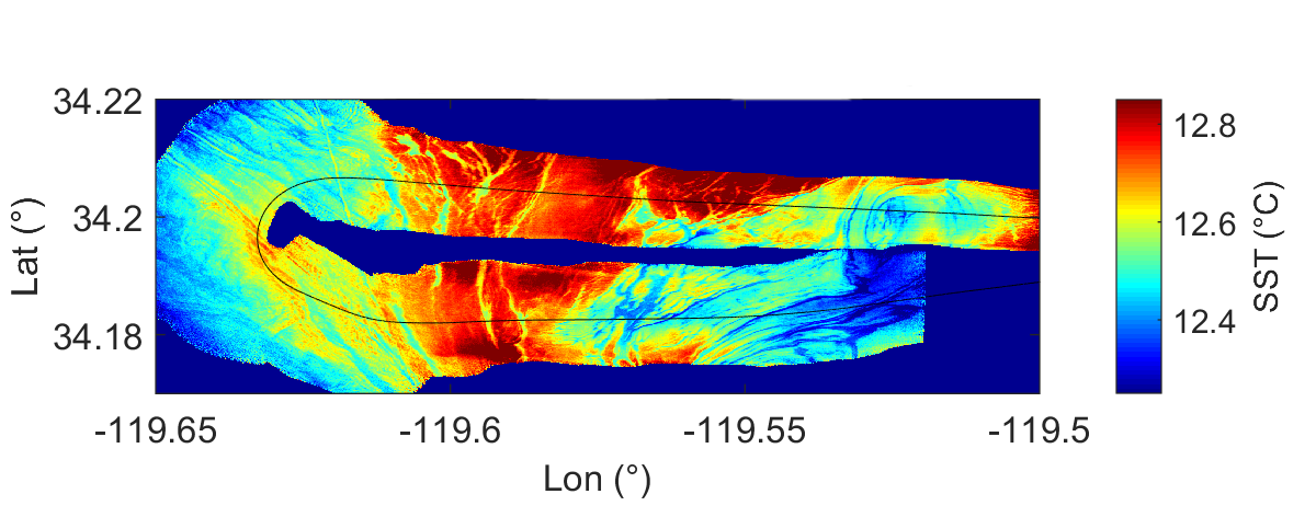
Airborne IR brightness temperature map collected over the ocean off the coast of California. Image courtesy Louis Marié#
▶ Advantages and limitations
Advantages
Non invasive SST measurements
Large area measurements
High frame rate (50 Hz)
Limitations
SST only
Cameras are expensive [100:150000]€
Inexpensive sensor such as MLX9064*, is affordable but require technical work.
Complex technology to handle : all the components must be carefully chosen, understood and handle with care. The orientation also affect the measurement.
Low industrial absolute accuracy (2°C) - may be corrected by post-processing
▶ References
You can access publications and book references via the library’s search tool.
Publications
Briggs, Martin A., Kevin E. Jackson, Fiona Liu, Eric M. Moore, Alaina Bisson, and Ashley M. Helton. 2022. “Exploring Local Riverbank Sediment Controls on the Occurrence of Preferential Groundwater Discharge Points” Water 14, no. 1: 11. doi
D. K. Hare, M. A. Briggs, D. O. Rosenberry, D. F. Boutt, J. W. Lane, 2015. A comparison of thermal infrared to fiber-optic distributed temperature sensing for evaluation of groundwater discharge to surface water, Journal of Hydrology, Volume 530, Pages 153-166, doi.
Websites
Teledyne, FLIR OEM, 2023. 12 Considerations for Thermal Infrared Camera Lens Selection, free download
Teledyne, FLIR, 2023. 7 things to know when selecting an IR camera for research & development, free download
Teledyne, FLIR, 2023, 8 things engineers should know about thermal imagine, free download
Infrared thermometer#
An infrared thermometer is an inexpensive alternative to measure SST at a single point. The measurement spot diameter depends on the distance-to-object ratio. The closer the sensor is to the surface, the smaller the measurement point (see instrument testo 830-T1 documentation for more information).
Instruments (such as pyrometers or medical IR thermometers) cost between 10-1000€. IR sensors can also be purchased separately and integrated into custom systems. Examples of IR sensors with 0.5°C accuracy (specified by the manufacturer) can be found for around 23 USD. A combination of measurements may help achieve better accuracy. [Zhang & Wang (2022)] propose a methodology to obtain SST measurements using integrated infrared thermometers, MLX90614 and Heitronics KT19. A more detailed methodology would be needed.
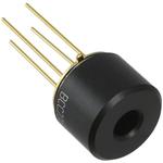
Temperature and humidity sensor MLX90614ESF-BCC-000-TU by Melexis website#
▶ Typical characteristics
Accuracy: [0.2°C-0.5°C] - see Melexis database
Time response: Instrument time response typically ranges from 0.5-1s (see RS website for examples). One must consider the time resolution of the full process as it will depends on the detector’s ability to adjust (the time constant for microbolometers is 12ms and is considered slow (“The Ultimate Infrared Handbook for R&D Professionals”)).
Sensitivity: To complete
Size : [3x3x1] - [9.1 x 17.2] mm - see Melexis database
Calibration: Need for multiple corrections
▶ Advantages and limitations
Advantages
Non-invasive measurement
Low cost IR sensor: sensor costs around $20
Small size (few mm diameter)
Limitations
One point measurement
Several sources of error
No publication about the sensor drift, sensitivity and accuracy
The accuracy specified by the manufacturer
▶ References
You can access publications and book references via the library’s search tool.
Zhang, Kailin, and Xinyu Wang. 2022. “High-Precision Measurement of Sea Surface Temperature with Integrated Infrared Thermometer” Sensors 22, no. 5: 1872. doi
Wikipedia
Historical and high-technology sensing techniques#
This section presents a non-exhaustive list of techniques that are either no longer used or represent high-tech solutions that are not well suited to DIY instruments. These techniques are included to privde insight into the evolution of oceanographic measurements techniques, and because some of them may become relevant again for low-tech development. Any contributions to completing these descriptions are more than welcome.
The following methods are covered:
Liquid dilatation: Mercury and alcohol thermometers used in early oceanography
Bimetallic strips: Temperature sensors based on differential thermal expansion of metals
Bathythermograph: Historical profiling instruments from the 1930s-1970s
Fiber optic sensing: Advanced optical techniques for subsurface temperature measurement
Sound velocity: Acoustic methods for indirect temperature measurement
▶ Liquid dilatation
Liquid-glass thermometers were used in early oceanography to measure temperature, for instance, on the Challenger expedition of 1872–1876. Reversing thermometers wee used on Niskin bottles to draw temperature profile [sect 16.4 from Lynne 2011].
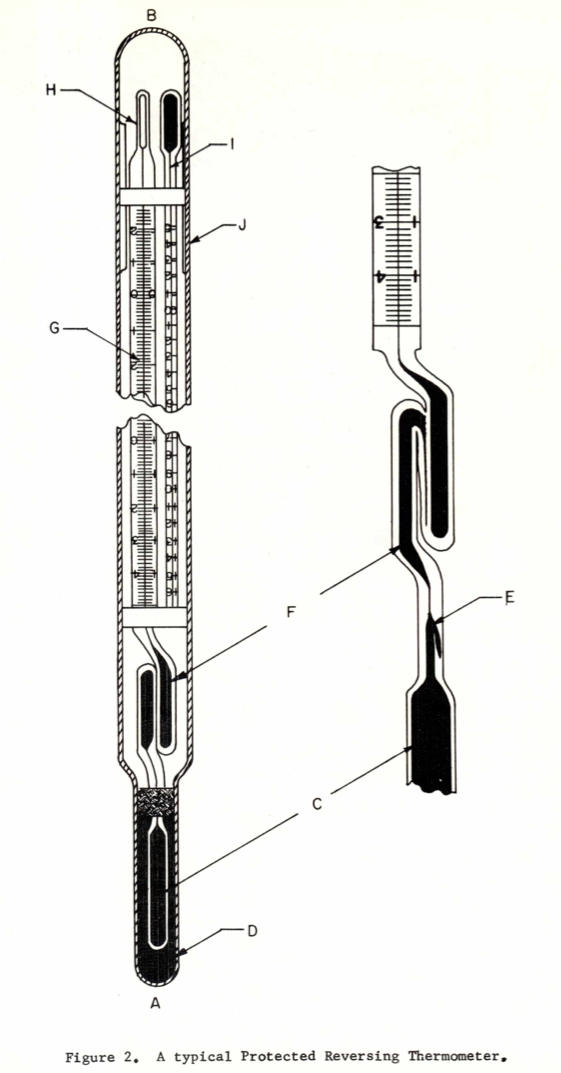
from Boyce (1996)#
Principle
The dilatation of a liquid at constant pressure is used to measure temperature changes. As the liquid temperature changes, its volume also changes. This dilation allows temperature measurement, such as in mercury or alcohol in-glass thermometers. Mercury expands in a near-linear manner, making it the most commonly used liquid.
Measurement process
The thermometer is lowered into the ocean. At a given depth, a reversing mechanism separates the mercury in the stem from the reservoir and captures the measurement [sect 1.3.1 from Emery and Thomson 2001].
Advantages and limitations
Advantages:
Accuracy can be better than 0.01°C (0.005°C in situ given in [Boyce 1996])
No energy needed
Limitations:
Slow measurements : 17.4 s response time [Emery 2001]
High pressure could deform or crush the thermometer
References
You can access publications and book references via the library’s search tool.
Scientific report
F. M. Boyce 1996. A brief study of the accuracy of the protected deep-sea reversing thermometer - Fisheries research board of canada, N°227. free pdf
Book
W. J. Emery & R. E. Thomson, 2001. Data Analysis Methods in Physical Oceanography - Elsevier Science, Revised Second Edition, ISBN 978-0-444-50756-3
Lynne D. Talley, George L. Pickard, William J. Emery, James H. Swift, 2011. Chapter S16 - Instruments and Methods, Editor(s): Lynne D. Talley, George L. Pickard, William J. Emery, James H. Swift, Descriptive Physical Oceanography (Sixth Edition), Academic Press, Pages 1-83, ISBN 9780750645522, pdf.
▶ Bimetallic strip
The bimetallic strip mechanism converts thermal energy into mechanical motion without requiring any external power source. A bimetallic strip is usually combined with other thermal component such as thermostat. Bimetallic strip was initially used in early marine chronometer. Today technology combine bimetallic strip In oceanography they can be combined with Fiber Bragg grating (FBG) to measure subsurface temperature and pressure [Anudeep Kumar Reddy et al. 2013].
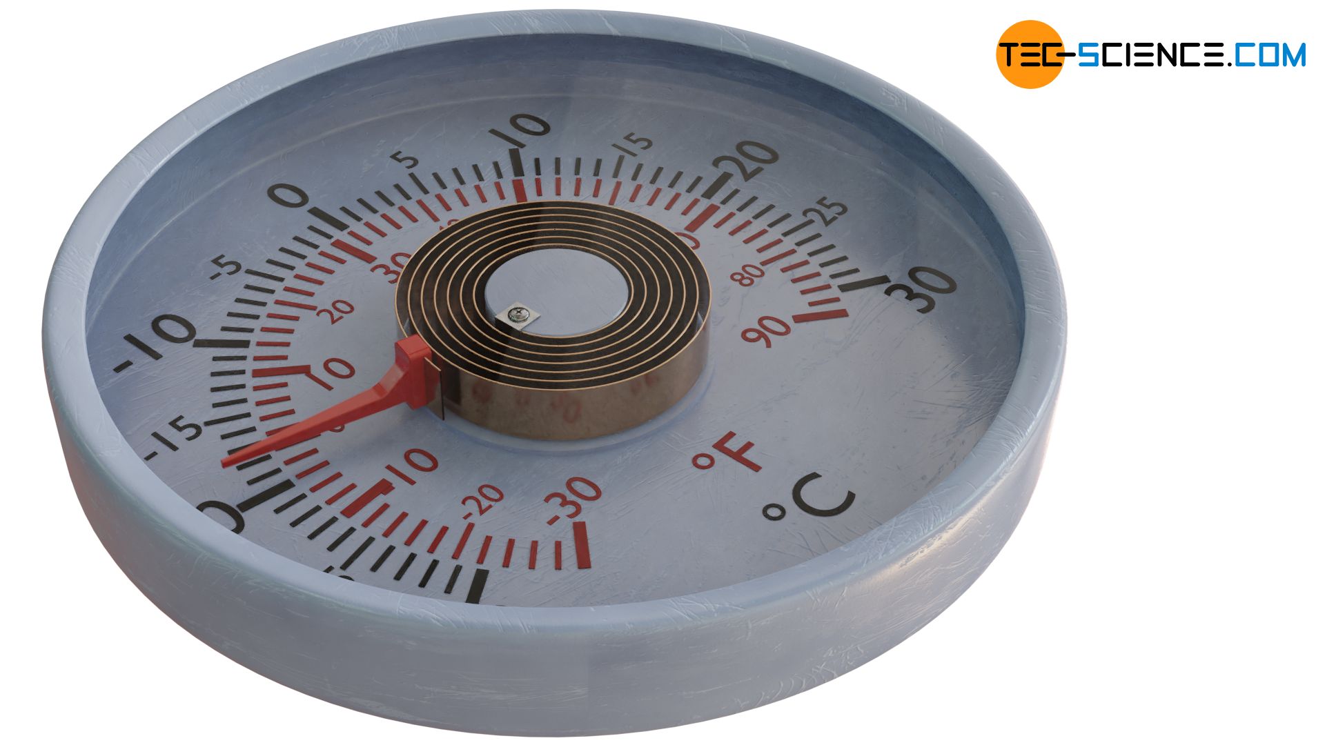
Illustration taken from Tec-Science website : How does a bimetallic strip thermometer work?#
Principle
A bimetallic strip consists of two metals with different coefficients of thermal expansion bonded together. When heated, the strip bends due to the difference in expansion rates.
Measurement process
The bending of the strip is used to actuate mechanical devices or measure temperature.
References
You can access publications and book references via the library’s search tool.
Publication
I. V. Anudeep Kumar Reddy, P. Saidi Reddy, G. R. C. Reddy, R. L. N. Sai Prasad, A. V. Narasimha Dhan, K. Sandeepkumar, and Sanjeev Afzulpurkar “Simultaneous measurement of temperature and pressure sensor for oceanography using Bragg gratings”, Proc. SPIE 8724, Ocean Sensing and Monitoring V, 87240Z (3 June 2013); doi
Website
https://www.tec-science.com/thermodynamics/temperature/how-does-a-bimetallic-strip-thermometer-work/
▶ BathyThermographs
The bathythermograph was developed in 1938 and extensively used from the 1930s to 1970s for measuring temperature profiles with depth. For the first time, an instrument recorded continuous profiles rather than discrete point measurements. During WWII, BT measurements were used to predict sonar range. More than 1,300,000 temperature-depth profiles have been acquired using this method [Couper & Lafond 1970].
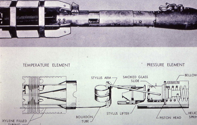
Mechanical BathyThermograph (MBT or BT) exploded view, Source: Neumann and Pierson (1966).#
The initial mechanical bathythermographs (Figure MBT) were then replaced by expendable bathythermographs (XBT) (Figure XBT). XBT allowed for the first synoptic view of the Japan/East Sea thermocline structure [Gordon et al. 2002]. Nowadays, XBT data are still used in oceanographic studies (see the NOAA/AOML XBT Network). XBTs are also used by volunteer observing ships [Sect 16.4.2.5 from Lynne 2011]. Similar objects were deployed in the atmosphere (see NOAA website).
eXpendable BathyThermograph (MBT or BT) exploded view, Source: NOAA website.#
Principle
To measure temperature profiles, the MBT operates on mechanical principles using the thermal expansion of xylene in capillary tubing. These mechanical movements are transferred through a linkage system to a stylus that traces curves on a smoked glass slide. The glass slide was moved at right angles with respect to the stylus by a pressure-sensitive bellows, creating a permanent record of temperature versus depth (Figure MBT). The MBT accuracy was excellent for the time as it could reach ±0.2 K and ±2 m with good calibration [sect 16.4.2.4 Lynne 2011], but doubtfully down to 0.06°C which was sometimes stated [sect 1.3.2 Emery 2001].
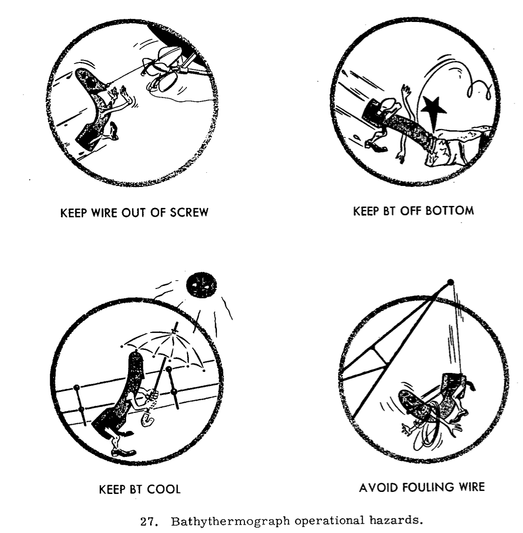
Illustration from the manufacturer’s instruction book - from [Couper et al. 1970].#
The MBT had numerous limitations. After retrieval, data were entered into files by hand and the opportunities for operator recording errors were considerable [Emery 2001]. The MBT was also restricted to depths less than 300 m and intended to be used with a ship traveling at a few knots maximum. The lowering and operating of the BT had to be done with care and loss of BTs was frequent (Figure BT hazard). The BT is a delicate instrument which would be easily damaged and danger points given in the instruction book were not to: “lower the BT while the ship is expected to turn;” “leave in a temperature greater than 105 °F;” “bump, drop or jar.” [Couper et al. 1970].
Nowadays the XBT uses a thermistor and electronic data acquisition system which reduced the MBT uncertainties and was able to go deeper (1500 m for XBT).
The different types of sensors
Standard MBT: Basic model for depths up to 285m
Deep MBT: Extended range version for depths up to 400m
Fine-structure MBT: Enhanced sensitivity for detecting small temperature variations
Expendable bathythermographs (XBT): Used thermistors which enhanced accuracy (around 0.1°C in laboratory) [Emery 2001].
Advantages and limitations
Advantages:
Continuous temperature-depth profiles
MBT : No electrical components to fail
Important historical dataset for climate studies
Limitations:
MBT : The data were entered into files by hand leading to opportunities for operator recording errors were considerable [Emery 2001]
Limited depth range
Ships must travel at no more than a few knots
Metal thermometers are subject to permanent deformation
References
You can access publications and book references via the library’s search tool.
Books
Lynne D. Talley, George L. Pickard, William J. Emery, James H. Swift, 2011. Chapter S16 - Instruments and Methods, Editor(s): Lynne D. Talley, George L. Pickard, William J. Emery, James H. Swift, Descriptive Physical Oceanography (Sixth Edition), Academic Press, Pages 1-83, ISBN 9780750645522, pdf.
W. J. Emery & R. E. Thomson, 2001. Data Analysis Methods in Physical Oceanography - Elsevier Science, Revised Second Edition, ISBN 978-0-444-50756-3
Scientific reports and publications
Couper, B. K. and Lafond, E. C, 1970. Mechanical bathythermograph, an historical review. Adv. Instrumn. Instrum. Soc. Am., 25, paper 735–70, PDF
Spilhaus, A. F., 1938: A bathythermograph. J. Mar. Res., 1, 95-100.
Gordon, A.L., C.F. Giulivi, C.M. Lee, H.H. Furey, A. Bower, and L. Talley. 2002. Japan/East Sea intrathermocline eddies. Journal of Physical Oceanography 32(6):1,960–1,974.
Websites
https://www.aoml.noaa.gov/hrd/about_hrd/HRD-P3_exp.html?print=yes- Neumann, G. and Pierson, W.J. (1966) Principles of Physical Oceanography. Prentice-Hall, Englewood Cliffs, 230-233.
▶Distributed Fiber Optic Sensing (DFOS)
Today fiber-optic cables are used as sensors for temperature, strain, and acoustic signals over the cable length. The system allow to map temperature anomaly along a cable at rest on the seafloor. The different technologies are Distributed acoustic sensing (DAS) with a sensitivity down to \(10^{-3}K\); Distributed Temperature Sensing (DTS) and Distributed Strain and Temperature Sensing (DSTS) and rely on Raman and Brillouin spectroscopy [Quiñones et al. 2023].

A cross section of the shore-end of a modern submarine communications cable. 1 – Polyethylene 2 – Mylar tape 3 – Stranded steel wires 4 – Aluminium water barrier 5 – Polycarbonate 6 – Copper or aluminium tube 7 – Petroleum jelly 8 – Optical fibers. Illustration by Oona Räisänen, from Submarine communications cable wikipedia#
References
Pelaez Quiñones, J.D., Sladen, A., Ponte, A. et al. High resolution seafloor thermometry for internal wave and upwelling monitoring using Distributed Acoustic Sensing. Sci Rep 13, 17459 (2023). doi
▶ Acoustic thermometry
Acoustic thermometry is widely used to measure atmospheric boundary layer characteristics or air characteristics in indoor environments [Arnold et al. 1999; Othmani et al. 2023]. In the ocean, acoustic thermometry allows for deep temperature measurements with 0.1°C precision at 500-1500 m [Woolfe et al. 2015]. The current description covers a range of different technologies. Any contributions with clarification and organization is welcome.
Thermometry is part of ocean acoustic tomography measurements, which were first developed based on theoretical work for ocean monitoring down to the mesoscale [Munk & Wunsch 1979; Behringer et al. 1982; ATOC technical report]. Thermometry initially required an acoustic emitter within the ocean, which was suspected to impact marine life [New York Times archive] but was demonstrated to be harmless to marine life, especially compared to boats [ATOC]. Later, it was demonstrated that passive measurements were sufficient to measure temperature changes [Woolfe et al. 2015]. Passive ocean acoustic thermometry (POAT) observations showed 0.007°C/year warming around 900 m over twenty years [Läslo et al. 2015]. Coastal thermometry is more challenging due to high-frequency changes in ocean characteristics and internal waves. Current work on vertical profiles of sound speed variations in coastal oceans presents measurements with 25 ms accuracy and 1 m vertical resolution even in the presence of linear and nonlinear internal waves [Tan et al. 2021].
Principle
Sound velocity in water changes with temperature, salinity, and pressure.
Measurement process
Acoustic sensors emit sound waves and measure their travel time or frequency shift. The sound velocity is calculated and correlated with temperature using established relationships.
The different types of methodology
Two main methodologies are used to measure sound variations in the ocean. The first method developed consists of measuring the propagation of acoustic signals between sources and receivers, refered to as Active Thermometry of Ocean Climate [ATOC]. The second method is Passive Ocean acoustic Thermometry which use ambient noise correlation [Woolfe et al 2015; Howe et al. 2019].
Advantages and limitations
Advantages:
Can measure temperature changes over entire ocean basins
Deep ocean measurement with 0.1°C accuracy
POAT is non invasive
Limitations:
Long term signal required to obtain the averaged sound speed, this seems to be improved by machine learning [Li et al. 2021]
Limited by acoustic propagation conditions
References
You can access publications and book references via the library’s search tool.
Papers :
K. Arnold, A. Ziemann, A. Raabe, 1999. Acoustic tomography inside the atmospheric boundary layer, Physics and Chemistry of the Earth, Part B: Hydrology, Oceans and Atmosphere, Volume 24, Issues 1–2, 1999,doi.
Behringer, D., Birdsall, T., Brown, M. et al. A demonstration of ocean acoustic tomography. Nature 299, 121–125 (1982). doi
Howe Bruce M. , Miksis-Olds Jennifer , Rehm Eric , Sagen Hanne , Worcester Peter F. , Haralabus Georgios ; Observing the Oceans Acoustically; Frontiers in Marine Science, Volume 6 - 2019, doi
Läslo G. Evers; Decadal observations of deep ocean temperature change passively probed with acoustic waves. JASA Express Lett. 1 July 2025; 5 (7): 076001. doi
F. Li, Kai Wang, Xishan Yang, Bo Zhang, Yanjun Zhang, Passive ocean acoustic thermometry with machine learning, Applied Acoustics, Volume 181, 2021, 108167, ISSN 0003-682X, doi.
W. Munk, C. Wunsch (1979). Ocean acoustic tomography: a scheme for large scale monitoring, Deep Sea Research Part A. Oceanographic Research Papers, Volume 26, Issue 2, Pages 123-161, ISSN 0198-0149, doi.
C. Othmani, N. S. Dokhanchi, S. Merchel, A. Vogel, M. E. Altinsoy, C. Voelker, F. Takali, 2023. Acoustic tomographic reconstruction of temperature and flow fields with focus on atmosphere and enclosed spaces: A review, Applied Thermal Engineering,doi.
Woolfe, K. F., Lani, S., Sabra, K. G., and Kuperman, W. A. (2015). “Monitoring deep-ocean temperatures using acoustic ambient noise,” Geophys. Res. Lett. 42(8), 2878–2884, https://doi.org/10.1002/2015GL063438
Tsu Wei Tan, Oleg A. Godin; Passive acoustic characterization of sub-seasonal sound speed variations in a coastal ocean. J. Acoust. Soc. Am. 1 October 2021; 150 (4): 2717–2737. https://doi.org/10.1121/10.0006664
Technical report
Sensors database#
This table lists the basic components of temperature sensor, not the instruments themselves. You can access a list of low-cost and DIY temperature instruments on the Scoop Ocean website.
• Drag & Drop: Click and drag column headers to reorder columns
• Links: URLs are converted to clickable link (🔗) icons
| Technology ⇄ | Type ⇄ | Sensor name ⇄ | Brands ⇄ | Detailed ⇄ | Datasheet URL ⇄ | Range ⇄ | Accuracy ⇄ | Sensitivity/resolution ⇄ | Response Time ⇄ | Dimensions ⇄ | Cost (1 unit) ⇄ | Where to buy? ⇄ | Drift & self heating ⇄ | Mechanical integration ⇄ | Electronical integration ⇄ | Associated instruments ⇄ | Related development tools ⇄ |
|---|---|---|---|---|---|---|---|---|---|---|---|---|---|---|---|---|---|
| 🌡️ Thermistor | Sensor | TSYS01 | TE Connectivity | TSYS digital temperature sensor. It includes a temperature sensing chip and a 24-bit ΔΣ-ADC. | 🔗 | -5°C - 50°C | 0.1°C | 0.01°C (for 3.3V) | 1 second (with 0.5 m/s flow) and 2 seconds (in still water). | 4x4x0.85 mm | 2-6 USD | — | — | — | — | Blue robotics Temperature Sensor (I2C) | 🔗 |
| 🌡️ Thermistor | Sensor | DS18B20 | FocuSens | Can refers either to the discrete sensors either to the probe assemblies | 🔗 | -55°C - 125°C | 0.5°C (constructor) 0.1°C (Open CTD project) | — | 0.75 s (constructor) : 5.7-8.5 s (Open CTD) | — | 6 USD | 🔗 | 0.2°C drift on a 1000h stress test at 12°C with V=5.5V | — | 🔗 | Waterproof DS18B20 Digital Temperature Sensor SKU DFR0198 | 🔗 |
| 🌡️ Thermistor | Sensor | ADT7320 | Analog Devices Inc. | Catalogue | 🔗 | -10°C - 85°C | 0.20°C (constructor) - 0.1°C (test Mastodon) | 0.0073°C | <2 s | 4x4x0.8 mm | 8-10 EUR | 🔗 | 0.0073°C | — | — | MASTODON mooring system | 🔗 |
| 🌡️ Thermistor | Sensor | FP07DB154N | Thermometrics | Small diameter glass-coated thermistor | 🔗 | 25°C-125°C | 0.01°C | <1.10^{-4}°C | 7 ms (constructor) - 11 ms (sect.2.15 Baumert 2005) | 2.2 x 12.7 mm | 158 EUR | 🔗 | « Lacks long term stability » [Wolk et al. 2002] | — | — | TurboMAP | 🔗 |
| ⚡ RTD | Sensor | PT100 | Adafruit | Platinum RTD : 3 wires 1 meter long | 🔗 | -50°C - 280°C | 0.5°C | 0.385Ω/°C | 0.15 s (with 0.4 m/s flow) | — | 11 USD | — | Self heating 0.4K/mW at 0°C | — | — | — | — |
| ⚡ RTD | Sensor | RS PRO Pt100 | RS Pro | RS PRO Pt100 Platinum Resistance Thin Film Detector | 🔗 | -50° - 250°C | — | — | — | — | 31.29 EUR | — | ±0.05% and self heating <0.5°C/mW | — | — | — | — |
| 🔥 Thermocouple | Sensor | CHCO | Omega | Type E bare wire butt-welded thermocouples | 🔗 | — | 0.75 mK (after amplification) | — | <0.8 ms | 0.65 mm diameter | ~10 EUR | — | — | — | — | Thermocouple Probe for High-Speed Temperature | 🔗 |
| 📡 IR Thermometer | Sensor | MLX90614 | Melexis | 1 point measurement | 🔗 | -40°C - 85°C | 0.5°C (room temperature) 0.2°C around human body T°C | 0.02°C | — | <2cm diameter | 14 USD | 🔗 | — | — | — | High-Precision Measurement of Sea Surface Temperature with Integrated Infrared Thermometer by Zhang and Wang 2022 | 🔗 |
| 📷 Thermal Camera | Sensor | MLX90642 | Melexis | 32x24 pixel matrix | 🔗 | -40°C - 260°C | « nor warranty is provided by Melexis about its accuracy » | — | — | — | 20 USD | 🔗 | — | — | — | — | — |
| 📋 Catalogue | Sensor list | — | Mouser Electronics | discrete sensors and probe assemblies (NTC, PTC, RTD, thermocouple, IR) | 🔗 | — | — | — | — | — | — | — | — | — | — | — | — |
| 📋 Catalogue | Sensor list | — | Guilcor | discrete sensors and probe assemblies (NTC,PTC and RTD) : on quotation | 🔗 | — | — | — | — | — | On quotation | — | — | — | — | — | — |
| 📋 Catalogue | Sensor list | — | Little fuse | discrete sensors and probe assemblies (NTC, PTC and RTD) | 🔗 | — | — | — | — | — | <50 EUR | 🔗 | — | — | — | — | — |
| 📋 Catalogue | Sensor list | — | RS | discrete sensors and probe assemblies (NTC, PTC, RTD, thermocouple, IR) | 🔗 | — | — | — | — | — | — | — | — | — | — | — | — |
| 📋 Catalogue | Sensor list | — | RobotShop | — | 🔗 | — | — | — | — | — | — | — | — | — | — | — | — |
| 📋 Catalogue | Sensor list | — | DFRobot | — | 🔗 | — | — | — | — | — | — | — | — | — | — | — | — |